codescan
Data ManagementScan wide-format code variables for pattern matches
Version 1.1.2 | 2026-05-30
codescan scans wide-format code slots (such as dx1–dx30 or proc1–proc20) with anchored regex or prefix rules and creates condition indicators, counts, or patient-level summaries — all without reshaping your data. codescan_describe is the reconnaissance companion: it shows what codes are actually present before you commit to a scanning rule set.
What it does
You tell codescan which code patterns to look for and what to name each condition. The command scans every code slot on every row, marks which conditions are present, and returns a summary with prevalence and Wilson confidence intervals. You can:
- Stay at the row level (one 0/1 indicator per encounter per condition)
- Collapse to one row per patient with
collapse - Merge patient-level results back onto encounter rows with
merge - Apply time windows relative to a reference date
- Compute Charlson, Elixhauser, or custom weighted scores
- Export prevalence tables and co-occurrence matrices to
.xlsxor.csv
It works with any string code system: ICD-10, ICD-9, KVÅ, CPT, ATC, OPCS, or proprietary codes.
Requirements
- Stata 16 or later
- No external package dependencies
Installation
capture ado uninstall codescan
net install codescan, from("https://raw.githubusercontent.com/tpcopeland/Stata-Tools/main/codescan") replace
The bundled example codefiles are installed with the package and can be used by
basename in codefile(). If you want editable local copies in the current
working directory, download them with:
net get codescan, from("https://raw.githubusercontent.com/tpcopeland/Stata-Tools/main/codescan") replace
Commands
| Command | Description |
|---|---|
codescan |
Scan wide-format code variables and generate indicators, counts, summaries, or scores |
codescan_describe |
Inspect the raw code inventory before writing scan rules |
Bundled Example Codefiles
| File | Purpose |
|---|---|
charlson_icd10_example.csv |
Charlson ICD-10 definitions with Quan et al. (2011) weights |
elixhauser_icd10_example.csv |
Elixhauser ICD-10 definitions with van Walraven et al. (2009) weights |
These can be requested directly by basename in codefile() — no path needed.
How It Works
The recommended workflow has four steps:
- Inspect the code inventory with
codescan_describe. This shows which codes and chapter prefixes actually occur in your data, and suggests patterns to target. - Draft simple rules with
define()and check the row-level results. At this stage the created variables appear alongside the original data so you can verify matches. - Choose the output shape. Stay row-level for auditing,
collapseto one row perid(), ormergepatient-level summaries back to encounter rows. - Add advanced features last. Once basic matches look right, layer on time windows (
lookback()/lookforward()), date summaries (alldates), hierarchy rules, scoring, and export/save options.
Which Variables to Scan
The words between codescan and the comma are a normal Stata varlist: they tell codescan which columns contain codes. The rules in define() or codefile() are then applied to every variable in that varlist.
codescan dx1 dx2 dx3, define(dm2 "E11")
codescan dx1-dx30, define(dm2 "E11")
codescan dx*, define(dm2 "E11")
codescan dx1-dx30 proc1-proc20, define(dm2 "E11" | proc "XF001")
Use explicit names (dx1 dx2 dx3) when there are only a few variables. Use a range (dx1-dx30) when the variables sit next to each other in the dataset order. Use a wildcard (dx*) when all variables with that prefix should be scanned. You can mix groups in one varlist when the same definitions should be checked across all of them.
If diagnosis codes, procedure codes, and medication codes need different dictionaries, run separate scans and use generate() so the output names do not collide:
codescan dx1-dx30, define(dm2 "E11" | htn "I1[0-35]") generate(dx_)
codescan proc1-proc20, define(mammo "XF001|XF002" | colectomy "JFB|JFH") ///
    mode(prefix) generate(proc_)
For troubleshooting, add detail to see how many matches came from each scanned variable. codescan_describe dx1-dx30 is for inventory: it pools the nonempty codes across the listed variables so you can decide what rules to write.
Regex Patterns in Plain English
mode(regex) is the default. For each code value, codescan uses Stata's regexm() function and automatically adds a start-of-string anchor. That means define(dm2 "E11") is checked like regexm(code, "^(E11)"): the code must start with E11.
Common patterns:
"E11"matchesE110,E119, andE11.9; it does not matchAE11."I1[0-35]"matchesI10,I11,I12,I13, andI15. The brackets mean "one character from this set";[0-35]means0,1,2,3, or5."E1[01]"matchesE10andE11."C7[7-9]|C80"matchesC77,C78,C79, orC80. A|inside a quoted regex pattern means "or".
The unquoted | in define() has a different job: it separates conditions.
* Two conditions: dm2 and htn
codescan dx1 dx2, define(dm2 "E11" | htn "I1[0-35]")

* One condition with two regex alternatives: metastatic
codescan dx1 dx2, define(metastatic "C7[7-9]|C80")
Use ~ for exclusions. This keeps the broad rule readable while removing specific subcodes:
codescan dx1 dx2, define(dm2 "E11" ~ "E116")
In mode(prefix), regex metacharacters are not special. The pattern is treated as one or more simple starts-with tokens separated by |, so "XF001|XF002" means "starts with XF001 or starts with XF002".
Choosing the Output Shape
| Goal | Use | What remains in memory |
|---|---|---|
| Check whether rules match the right encounters | No collapse or merge |
Original rows plus condition variables |
| Build an analysis dataset with one row per patient | id(pid) collapse |
One row per id() |
| Keep encounter rows but attach patient-level flags | id(pid) merge |
Original rows plus patient-level results |
| Keep the original data untouched and store results separately | frame(results) replace |
Original data plus a new frame |
| Save the transformed dataset to disk | saving(results.dta, replace) |
Same data as the selected output shape |
| Save the prevalence summary table | export(results.xlsx) or export(results.csv) |
Data in memory are unchanged by the export |
For most analytic workflows, start with row-level output while checking the
rules, then use collapse once the definitions are stable.
Worked Examples
1. Build a small toy dataset
codescan is designed for wide-format code slots, so the examples use a compact inline dataset representing five encounters for three patients, with diagnosis codes, a procedure code, and dates.
clear
input long pid str6 dx1 str6 dx2 str6 proc1 double visit_dt double index_dt
1 "E110" "I10"  "XF001" 21914 21915
1 "Z00"  "E119" ""      21880 21915
2 "I50"  ""     "JFB10" 21900 21915
2 "E102" ""     ""      22020 21915
3 "Z00"  ""     ""      21910 21915
end
format visit_dt index_dt %td
2. Inspect the code inventory before writing rules
Start here when you do not yet know which prefixes or patterns are in the raw data. codescan_describe tabulates unique codes across wide-format variables, showing the top N by frequency and a chapter summary grouped by first character.
codescan_describe dx1 dx2, top(10)
You can also save a draft CSV codefile from the chapter summary:
codescan_describe dx1 dx2, save(chapter_rules.csv)
3. Start with a row-level scan
This is the simplest use case. It creates one 0/1 output variable per named condition. Keep the first pass simple and verify the matches before adding windows or patient-level aggregation.
codescan dx1 dx2, define(dm2 "E11" | htn "I1[0-35]" | chf "I50")
After this command, dm2 is 1 on rows where dx1 or dx2 starts with E11; htn is 1 where either slot starts with I10, I11, I12, I13, or I15; and chf is 1 for I50*.
4. Collapse to one row per patient with a lookback window
Once the rule set looks right, add IDs and dates. lookback(365) limits matches to the prior year relative to refdate(), and alldates requests _first, _last, and _count date-summary variables for each condition.
codescan dx1 dx2, id(pid) date(visit_dt) refdate(index_dt) ///
    define(dm2 "E11" | htn "I1[0-35]" | chf "I50") ///
    lookback(365) inclusive collapse alldates
5. Use exclusion patterns
Use ~ after the inclusion pattern to exclude specific codes. Here dm2 matches all E11* codes except E116:
codescan dx1 dx2, define(dm2 "E11" ~ "E116" | htn "I1[0-35]")
6. Prefix matching for procedure codes
regex is the default. Switch to mode(prefix) when simple starts-with logic is enough and you do not need regex features. Pipe-separated tokens are alternative prefixes.
codescan proc1, define(mammo "XF001|XF002" | colectomy "JFB|JFH") mode(prefix)
7. Save reusable definitions, then load them back as a codefile
This is the transition from ad hoc rule drafting to a reusable dictionary workflow. save() writes the parsed define() rules to a CSV, and codefile() reads them back.
codescan dx1 dx2, define(dm2 "E11" | htn "I1[0-35]") save(dm_rules.csv)
codescan dx1 dx2, codefile(dm_rules.csv)
8. Compute a Charlson score from the bundled example codefile
The bundled example names are recognized directly by codefile() — no path needed. hierarchy() zeroes out the less-severe condition when both members of a pair are present, before scoring.
codescan dx1 dx2, codefile(charlson_icd10_example.csv) id(pid) collapse ///
    score(charlson) ///
    hierarchy(dm_comp > dm_uncomp \ liver_severe > liver_mild \ metastatic > cancer)
After this command, each patient has a _score variable containing the weighted Charlson comorbidity index.
9. Non-destructive workflow with frames
frame() stores the collapsed result in a named frame, leaving the original data untouched. This is the recommended pattern when you need both encounter-level data and a patient-level summary in the same session.
codescan dx1 dx2, define(dm2 "E11" | htn "I1[0-35]") id(pid) collapse ///
    frame(results) replace
frame results: list
10. Export a summary table and save the result dataset
Use export() for the prevalence table and saving() for the transformed dataset. format() controls the number format in both the console output and the exported file.
codescan dx1 dx2, define(dm2 "E11" | htn "I1[0-35]") id(pid) collapse ///
    export(codescan_results.xlsx) ///
    saving(codescan_results.dta, replace) ///
    format(%9.2f)
11. Merge patient-level results back to original rows
merge computes patient-level summaries and joins them back, so every row for a given patient gets the same comorbidity values.
codescan dx1 dx2, define(dm2 "E11" | htn "I1[0-35]") id(pid) merge
12. Multi-window sensitivity analysis
Supply several lookback values to compare how prevalence changes across windows. r(sensitivity) returns a matrix of prevalences by condition and window.
codescan dx1 dx2, id(pid) date(visit_dt) refdate(index_dt) ///
    define(dm2 "E11" | htn "I1[0-35]") ///
    lookback(90 365) inclusive collapse
Demo
The demo uses synthetic administrative data: 500 patients with 3 encounters each, 4 wide-format ICD-10 diagnosis slots, and 1 procedure code variable.
Code inventory with codescan_describe
Console output (click to expand)
. noisily codescan_describe dx1 dx2 dx3 dx4, top(15)
codescan describe: 4 variables, 61 unique codes,      3,411 total entries

  Code             Frequency      Percent     Cumul %
  ----------------------------------------------------
  I110                    80         2.3%        2.3%
  C34                     71         2.1%        4.4%
  E114                    68         2.0%        6.4%
  G81                     67         2.0%        8.4%
  E119                    67         2.0%       10.3%
  E102                    66         1.9%       12.3%
  C85                     65         1.9%       14.2%
  C80                     65         1.9%       16.1%
  Z96                     64         1.9%       18.0%
  G820                    63         1.8%       19.8%
  I71                     63         1.8%       21.7%
  C79                     61         1.8%       23.5%
  M06                     61         1.8%       25.2%
  G311                    61         1.8%       27.0%
  K25                     61         1.8%       28.8%
  ... (46 more codes)

  By first character:
  Char         Codes     Entries
  ----------------------------------
  I               10         558
  C                9         527
  E                8         488
  K                5         263
  G                4         238
  F                4         221
  D                4         217
  J                3         168
  M                3         167
  N                3         161
  Z                3         160
  B                3         153
  R                2          90

  Suggested patterns:
    define(chapter_I "I") — 10 codes, 558 entries
    define(chapter_C "C") — 9 codes, 527 entries
    define(chapter_E "E") — 8 codes, 488 entries
    define(chapter_K "K") — 5 codes, 263 entries
    define(chapter_G "G") — 4 codes, 238 entries
Inline define — row-level scan
. noisily codescan dx1 dx2 dx3 dx4,
>     define(dm "E1[01]" | htn "I1[0-35]" | chf "I50" | copd "J4[0-7]" |
>            cancer "C[0-7]" ~ "C77|C78|C79|C80" | metastatic "C7[789]|C80")
>     label(dm "Diabetes" \ htn "Hypertension" \ chf "Heart failure" \
>           copd "COPD" \ cancer "Cancer (non-met)" \ metastatic "Metastatic cancer")
>     detail noisily
  dm: 384 matches across 4 variables
  htn: 227 matches across 4 variables
  chf: 51 matches across 4 variables
  copd: 159 matches across 4 variables
  cancer: 212 matches across 4 variables
  metastatic: 171 matches across 4 variables

codescan: 6 conditions, 4 variables, N =      1,500

  Condition              Matches   Prevalence            [95% CI]
  ----------------------------------------------------------------
  dm                         384        25.6%    [ 23.5,  27.9]
  htn                        227        15.1%    [ 13.4,  17.0]
  chf                         51         3.4%    [  2.6,   4.4]
  copd                       159        10.6%    [  9.1,  12.3]
  cancer                     212        14.1%    [ 12.5,  16.0]
  metastatic                 171        11.4%    [  9.9,  13.1]

  Per-variable match contribution:
  dm: 129 in dx1, 96 in dx2, 100 in dx3, 59 in dx4
  htn: 84 in dx1, 47 in dx2, 45 in dx3, 51 in dx4
  chf: 16 in dx1, 10 in dx2, 13 in dx3, 12 in dx4
  copd: 51 in dx1, 31 in dx2, 39 in dx3, 38 in dx4
  cancer: 66 in dx1, 50 in dx2, 46 in dx3, 50 in dx4
  metastatic: 42 in dx1, 51 in dx2, 39 in dx3, 39 in dx4
Charlson scoring — full clinical workflow
Console output (click to expand)
. noisily codescan dx1 dx2 dx3 dx4,
>     codefile(charlson_icd10_example.csv)
>     id(pid) date(visit_dt) refdate(index_dt)
>     lookback(365) inclusive
>     collapse alldates countrows
>     score(charlson)
>     hierarchy(dm_comp > dm_uncomp \ liver_severe > liver_mild \ metastatic > cancer)
>     cooccurrence detail noisily
mi: 28 matches across 4 variables
chf: 44 matches across 4 variables
pvd: 39 matches across 4 variables
cvd: 0 matches across 4 variables
(note: condition cvd matched 0 observations)
dementia: 28 matches across 4 variables
copd: 40 matches across 4 variables
rheumatic: 45 matches across 4 variables
peptic: 14 matches across 4 variables
liver_mild: 44 matches across 4 variables
dm_uncomp: 62 matches across 4 variables
dm_comp: 61 matches across 4 variables
hemiplegia: 41 matches across 4 variables
renal: 65 matches across 4 variables
cancer: 98 matches across 4 variables
liver_severe: 28 matches across 4 variables
metastatic: 45 matches across 4 variables
hiv: 28 matches across 4 variables
(hierarchy: 3 rule(s) applied)
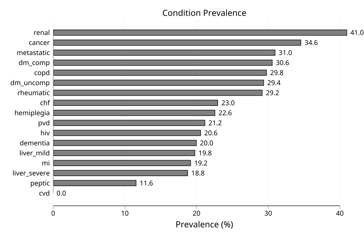
codescan: 17 conditions, 4 variables, N = 344
Window: 365 days before index_dt (inclusive)
Condition Matches Prevalence [95% CI]
----------------------------------------------------------------
mi 28 8.1% [ 5.7, 11.5]
chf 43 12.5% [ 9.4, 16.4]
pvd 37 10.8% [ 7.9, 14.5]
cvd 0 0.0% [ 0.0, 1.1]
dementia 28 8.1% [ 5.7, 11.5]
copd 39 11.3% [ 8.4, 15.1]
rheumatic 45 13.1% [ 9.9, 17.1]
peptic 14 4.1% [ 2.4, 6.7]
liver_mild 38 11.0% [ 8.2, 14.8]
dm_uncomp 53 15.4% [ 12.0, 19.6]
dm_comp 61 17.7% [ 14.1, 22.1]
hemiplegia 41 11.9% [ 8.9, 15.8]
renal 62 18.0% [ 14.3, 22.4]
cancer 85 24.7% [ 20.4, 29.5]
liver_severe 28 8.1% [ 5.7, 11.5]
metastatic 44 12.8% [ 9.7, 16.7]
hiv 28 8.1% [ 5.7, 11.5]
Collapsed to 344 unique pid values
charlson score: mean = 3.89, median = 3.0, range = [ 0, 17]
Co-occurrence: 17×17 matrix exported to codescan_results.xlsx
. summarize _score, detail
                       charlson score
-------------------------------------------------------------
      Percentiles      Smallest
 1%            0              0
 5%            0              0
10%            1              0       Obs                 344
25%            2              0       Sum of wgt.         344

50%            3                      Mean           3.892442
                        Largest       Std. dev.      3.062526
75%            6             13
90%            8             14       Variance       9.379068
95%            9             14       Skewness       1.024558
99%           13             17       Kurtosis       3.972026
Prevalence chart
Key Behaviors
- Anchored matching: patterns are anchored at the start of each code value.
define(dm2 "E11")matchesE110andE119, notAE11. - Default labels: if neither
label()nor a codefilelabelcolumn supplies a label, displayed and exported output use the condition name. - Regex vs. prefix:
mode(regex)(default) supports character classes and alternation.mode(prefix)uses simple starts-with comparisons and is usually faster. - Exclusion patterns: use
~after the inclusion pattern, e.g.define(dm2 "E11" ~ "E116"). Multiple exclusions are allowed:define(x "A" ~ "A1" ~ "A2"). - nodots: strips periods during matching without modifying the stored data.
- nocase: uppercases patterns and code values internally for case-insensitive matching.
- tostring: converts numeric code variables to string before scanning; original data are restored afterward.
- collapse vs. merge:
collapsecreates one row perid().mergeattaches patient-level results back to the original row structure. - alldates: shorthand for
earliestdate,latestdate, andcountdate. These create_first,_last, and_countdate-summary variables. - countrows: creates
_nrowsvariables counting the number of rows (not unique dates) with a qualifying match. Does not requiredate(). - countmode: changes created variables from 0/1 indicators to integer counts (number of code slots matched per row, summed across rows after collapse/merge).
- hierarchy: zeroes out inferior conditions when the superior is present. Written as
superior > inferior, separated by\. - generate: prefixes all created variable names, useful when running separate diagnosis, procedure, and medication scans on the same dataset.
- unmatched: creates a row-level 0/1 flag for observations that matched no condition.
- matched_code: creates a row-level variable holding the first code value that survived matching.
- frame: stores the result in a named frame and implies
preserve, so the original data are untouched. - Confidence intervals: prevalence CIs use the Wilson score method at the current
c(level)setting.
Definition Rules and Codefiles
Inline definitions use this structure:
define(name "inclusion_pattern" ~ "exclusion_pattern" | name2 "pattern2")
The inclusion and exclusion patterns are anchored at the start of each code
value. In default mode(regex), "I1[0-35]" matches I10, I11, I12,
I13, and I15. In mode(prefix), pipe-separated tokens are treated as
simple alternative prefixes.
There are three practical ways to list condition definitions:
- Keep a short rule set inline with
define(). - Put many conditions in a CSV or
.dtacodefile, with one row per condition. - Use
codescan_describe, save(chapter_rules.csv)orcodescan, save(rules.csv)to create a starter CSV, then edit it.
Definitions apply to all variables in the varlist. To use different definitions for different variable groups, run separate calls with generate() prefixes, as shown above.
Reusable codefiles may be CSV or Stata .dta files. Column names are matched
case-insensitively.
| Column | Required | Meaning |
|---|---|---|
name |
Yes | Valid Stata condition name; must be unique and no longer than 26 characters |
pattern |
Yes | Inclusion pattern or pipe-separated prefix list |
exclusion |
No | Exclusion pattern(s), combined with ` |
label |
No | Human-readable label for output variables and tables |
weight |
Only for score(custom) |
Numeric score weight |
Use save(rules.csv) to turn an inline define() rule set into a reusable
codefile. Use saving(results.dta, replace) for the final transformed dataset;
the two option names deliberately do different jobs.
Output Reference
codescan creates one variable per condition. Without countmode, those
variables are 0/1 indicators. With countmode, they are integer counts of
matching code slots. With collapse or merge, optional date/count variables
are added as requested:
| Option | Created variables |
|---|---|
earliestdate |
<condition>_first |
latestdate |
<condition>_last |
countdate |
<condition>_count for unique dates |
countrows |
<condition>_nrows for matching rows or code-slot hits under countmode |
| `score(charlson | elixhauser |
Important returned results include r(summary) with count, prevalence, and
Wilson confidence interval columns; r(codelist) with count and prevalence;
r(varcounts) when detail is used; r(cooccurrence) when cooccurrence is
used; and r(sensitivity) for multi-window lookback() analyses.
codescan_describe returns r(top_codes) with columns frequency, percent,
and cumul_pct, and r(chapters) with columns codes and entries. These are
useful for automated checks before freezing a code dictionary.
Troubleshooting
| Symptom | Likely cause and fix |
|---|---|
not a string variable |
Code variables were imported as numeric; add tostring or convert them before scanning |
collapse requires id() |
Patient-level output needs an identifier supplied through id() |
lookback()/lookforward() require both date() and refdate() |
Windowing needs an event date and a reference date, both stored as numeric Stata daily dates |
variable ... already exists |
Add replace only after confirming that overwriting existing output variables is intended |
| A condition matches zero observations | Check spelling, dots, case, anchoring, and whether mode(regex) or mode(prefix) matches the intended rule |
Multi-window lookback() fails |
Multiple windows require collapse or merge because the comparison is patient-level |
References
- Quan H, Sundararajan V, Halfon P, et al. (2005). ICD-9-CM and ICD-10 coding algorithms for defining comorbidities in administrative data.
- Quan H, Li B, Couris CM, et al. (2011). Updated Charlson comorbidity weights for risk adjustment.
- van Walraven C, Austin PC, Jennings A, Quan H, Forster AJ. (2009). A point-system adaptation of the Elixhauser comorbidity measure for hospital mortality.
Changelog
1.1.2 (2026-05-30)
- Fix: bundled helper files (
_codescan_codefile,_codescan_definitions,_codescan_hierarchy,_codescan_outputs,_codescan_score) now precede everyprogram definewithcapture program drop. Because the loader re-runs a whole helper file whenever any one of its programs is missing from memory, a partial-load state could otherwise crash a second in-session invocation withprogram ... already defined. All sub-programs are now idempotent on reload.
1.1.1 (2026-05-28)
- Fix:
matched_code()no longer captures codes from observations outside the primary analysis window when combined with a multi-windowlookback()andmerge. The supplementary sensitivity scan previously reused the matched-code buffer and populated it for secondary-window-only rows. - Docs: corrected the
codescan_describe.adoheader to list thesave()option and ther(top_codes)/r(chapters)matrices.
Author
Timothy P Copeland, Karolinska Institutet