eplot

Version 1.2.0 | 2026-06-06

eplot creates forest plots and coefficient plots from four sources — variables in memory, active or stored estimation results, preassembled matrices, and graph-ready frames — under one command with one set of options.

Quick Start

Run a regression and plot the coefficients in two lines:

sysuse auto, clear
regress price mpg weight foreign
eplot ., drop(_cons) cicap

That's it. eplot . reads the active estimation results and draws a coefficient plot with capped confidence intervals.

Requirements

• Stata 16 or later
• No external package dependencies

Installation

capture ado uninstall eplot
net install eplot, from("https://raw.githubusercontent.com/tpcopeland/Stata-Tools/main/eplot") replace

Commands

Command	Description
eplot	Draw effect plots from data in memory, estimation results, matrices, or graph-ready frames

How It Works

eplot detects its input mode automatically from the arguments you supply:

Call	Mode	When to use
eplot es lci uci, ...	Data	Effect sizes already in variables (meta-analysis, imported results)
eplot . or eplot m1 m2, ...	Estimates	Plot coefficients from a regression you just ran, or compare stored models
eplot, matrix(R) ...	Matrix	Results assembled in a Stata matrix
eplot, frame(F) ...	Frame	Results assembled in a graph-ready Stata frame, including tabtools eplotframe() output

Mode detection gives precedence to explicit frame() and matrix() calls, then to data mode when the first three tokens are numeric variables. In ambiguous cases, use eplot . to force estimates mode, matrix() to force matrix mode, or frame() to force frame mode explicitly.

Feature Highlights

• One command, four input modes — data in memory, estimation results, matrices, and graph-ready frames share one option vocabulary
• Tabtools bridge — plot frames emitted by regtab, effecttab, comptab, and hrcomptab through their eplotframe() options
• Journal style presets — style(lancet), style(jama), style(nejm), style(bmj) apply ready-made looks; override any individual element
• Multi-model comparison — overlay stored estimates side by side with modellabels(), offset(), and palette()
• Values annotation — add formatted effect text next to each marker with values; customize with vformat() and stars
• Significance coloring — sigcolors draws significant and non-significant effects in contrasting colors
• Grouped and annotated layouts — groups(), headers(), gap(), and favors() organize complex plots
• Meta-analysis support — prediction intervals (pi()), heterogeneity statistics (i2(), tau2(), qstat()), weighted boxes, and diamond pooled effects
• Eform with auto-labeling — eform exponentiates coefficients and sets the axis label automatically (Odds Ratio, Hazard Ratio, IRR)

Worked Examples

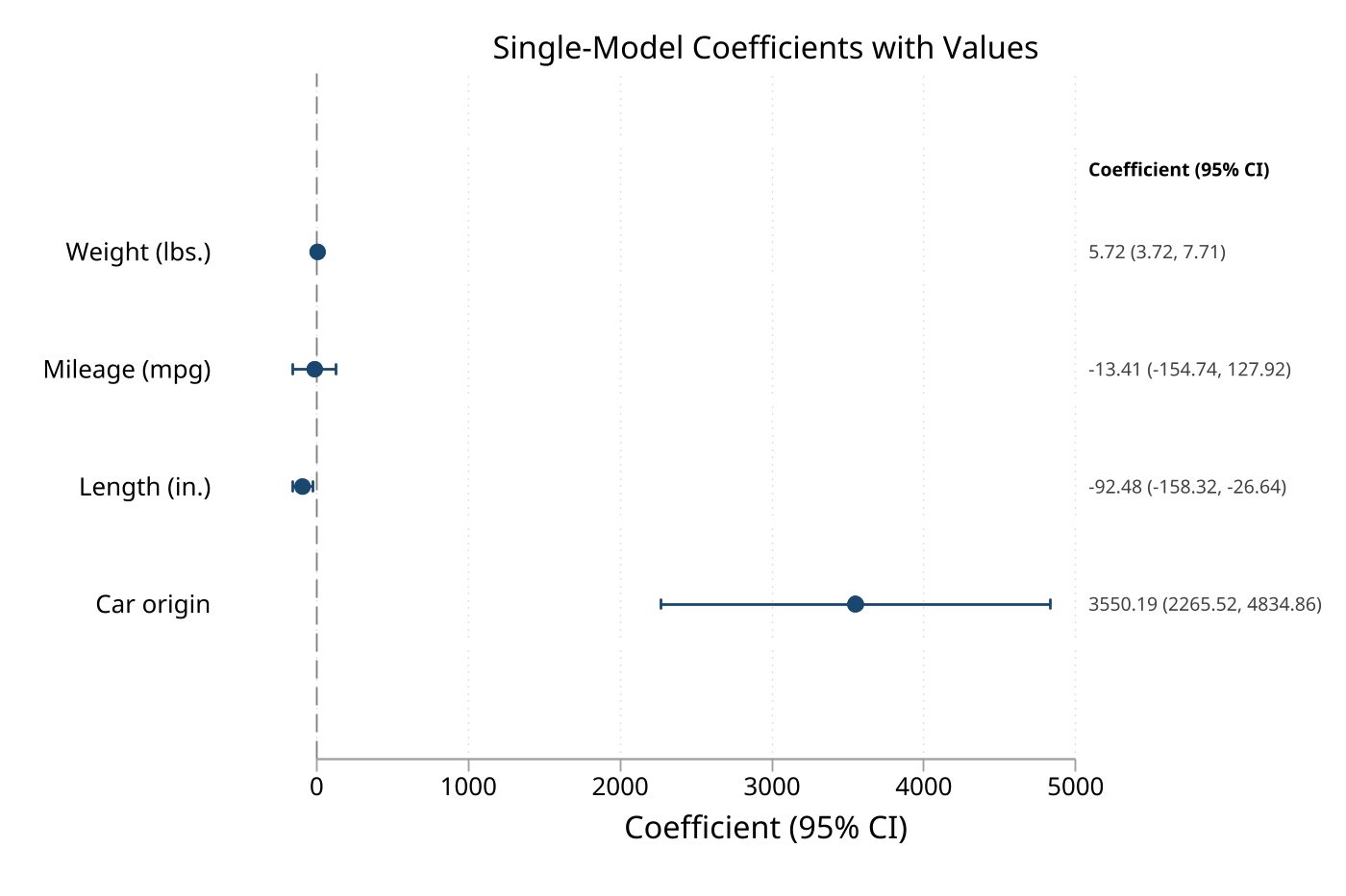
1. Coefficient plot with custom labels

The fastest way to use eplot — run a regression, then plot the results immediately.

sysuse auto, clear
regress price mpg weight foreign

eplot ., drop(_cons) ///
    coeflabels(mpg = "Miles per Gallon" ///
               weight = "Vehicle Weight" ///
               foreign = "Foreign Make") ///
    cicap values

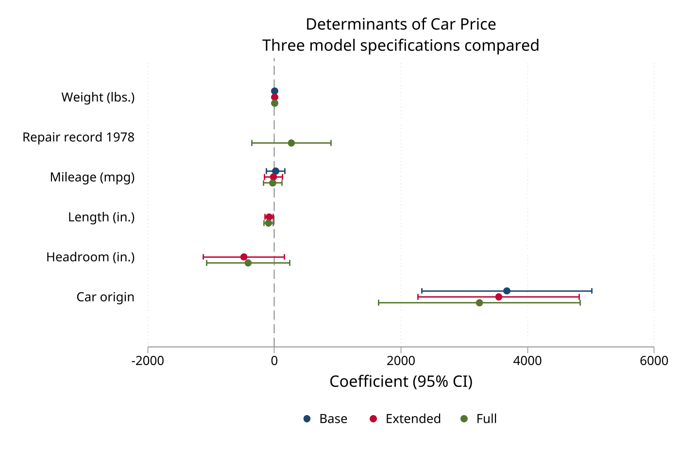
2. Compare two stored models

Multi-model estimates mode is useful when you want to compare a base model and an adjusted model side by side.

sysuse auto, clear

quietly regress price mpg weight foreign
estimates store base

quietly regress price mpg weight length foreign headroom
estimates store extended

eplot base extended, drop(_cons) ///
    modellabels("Base" "Extended") ///
    coeflabels(mpg = "Miles per Gallon" ///
               weight = "Vehicle Weight" ///
               length = "Body Length" ///
               headroom = "Headroom" ///
               foreign = "Foreign Make") ///
    cicap

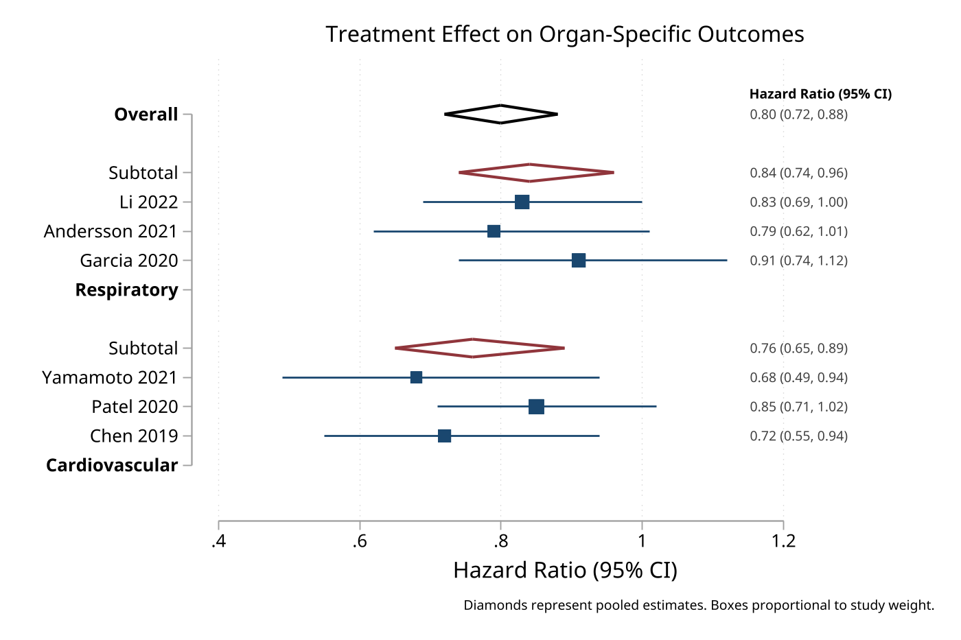
3. Forest plot from data in memory

Use data mode when you already have effect sizes and confidence limits in variables — for example, after a meta-analysis or when reading results from another system.

clear
input str20 study es lci uci weight
"Smith 2020"   -0.16  -0.36   0.03  15.2
"Jones 2021"   -0.33  -0.54  -0.12  18.4
"Brown 2022"   -0.09  -0.25   0.06  22.1
"Wilson 2023"  -0.39  -0.65  -0.12  12.8
"Overall"      -0.24  -0.34  -0.13   .
end

gen byte type = cond(study == "Overall", 5, 1)

eplot es lci uci, labels(study) weights(weight) type(type) ///
    values effect("Mean Difference (95% CI)")

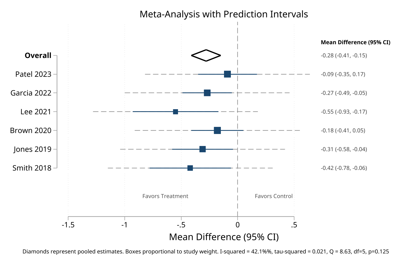
4. Meta-analysis forest plot with heterogeneity

Data mode supports prediction intervals and heterogeneity statistics for publication-ready meta-analysis plots.

clear
input str20 study es lci uci weight byte type
"Smith 2018"   -0.42  -0.78  -0.06  12.3  1
"Jones 2019"   -0.31  -0.58  -0.04  16.8  1
"Brown 2020"   -0.18  -0.41   0.05  21.5  1
"Lee 2021"     -0.55  -0.93  -0.17  10.2  1
"Garcia 2022"  -0.27  -0.49  -0.05  19.1  1
"Patel 2023"   -0.09  -0.35   0.17  20.1  1
"Overall"      -0.28  -0.41  -0.15   .    5
end

eplot es lci uci, labels(study) weights(weight) type(type) ///
    values vformat(%4.2f) ///
    i2("42.1") tau2("0.021") qstat("8.63, df=5, p=0.125") ///
    effect("Mean Difference (95% CI)")

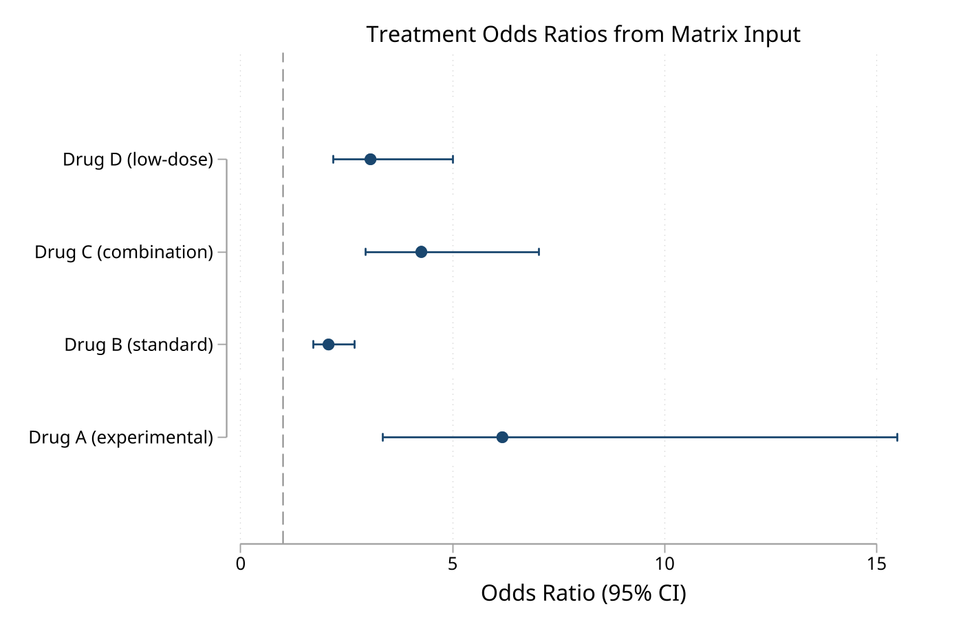
5. Plot from a matrix

Matrix mode is useful when the effect table is already assembled programmatically.

matrix R = (1.5, 1.1, 2.0 \ 0.8, 0.6, 1.2 \ 1.2, 0.9, 1.6)
matrix rownames R = "Treatment_A" "Treatment_B" "Treatment_C"

eplot, matrix(R) eform ///
    effect("Odds Ratio") ///
    values

6. Logistic regression with odds ratios

After a logistic model, eform exponentiates coefficients to odds ratios and sets the axis label automatically. Factor variables are labeled using Stata's value labels.

sysuse auto, clear
logit foreign mpg weight i.rep78
eplot ., eform cicap values

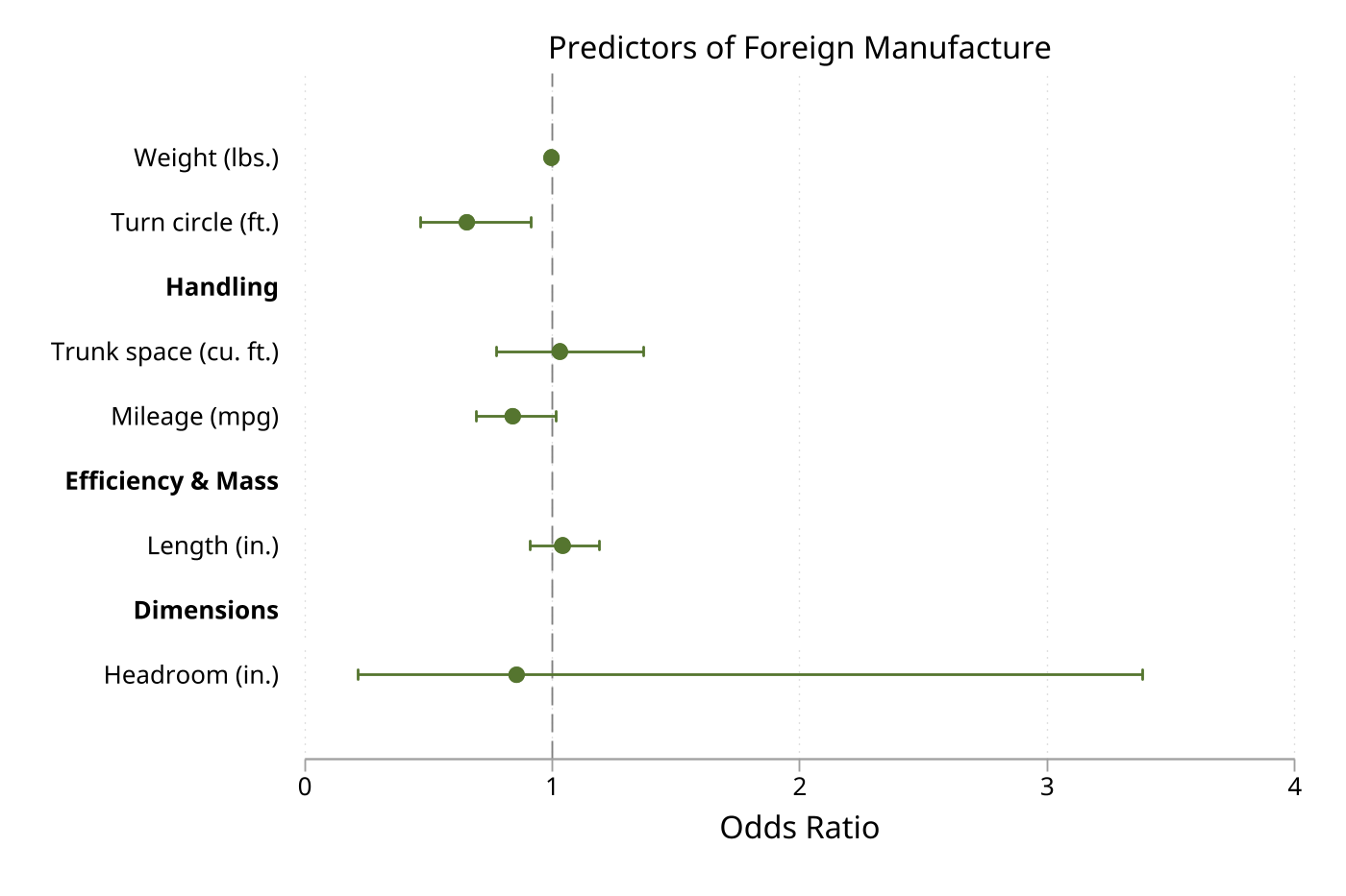
7. Grouped coefficients with significance coloring

Layer options to organize and annotate complex plots. groups() adds section headers, gap() adds space between groups, sigcolors highlights statistical significance, and stars adds asterisks.

sysuse auto, clear
regress price mpg weight length turn foreign rep78

eplot ., noconstant ///
    groups(mpg weight length turn = "Vehicle Characteristics" ///
           foreign rep78 = "Other Factors") ///
    gap(0.5) ///
    stars values sigcolors

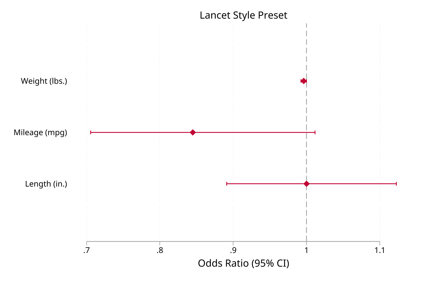
8. Journal style presets

Apply a journal-style preset, then override individual elements as needed.

sysuse auto, clear
regress price mpg weight foreign
eplot ., noconstant style(lancet)

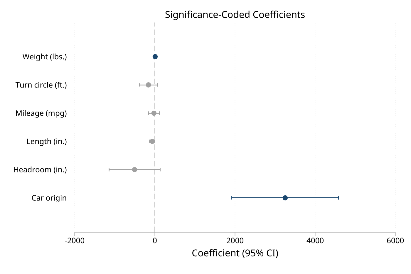
9. Significance coloring with custom colors

eplot ., noconstant sigcolors sigcolor(navy) insigncolor(gs12) cicap

10. Forest plot from a tabtools table

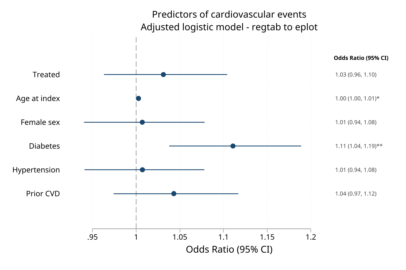
Frame mode reads the graph-ready companion frame that tabtools commands produce with eplotframe() — so a published regression table and its forest plot share one set of estimates. regtab writes the table and the frame together; eplot plots the frame.

collect clear
quietly collect: logistic cv_event treated index_age female diabetes hypertension prior_cvd
regtab, coef("OR") noint eplotframe(or_effects, replace)

eplot, frame(or_effects) labels(label) rowtype(rowtype) ///
    null(1) values stars vformat(%4.2f) ///
    effect("Odds Ratio (95% CI)") ///
    title("Predictors of cardiovascular events")

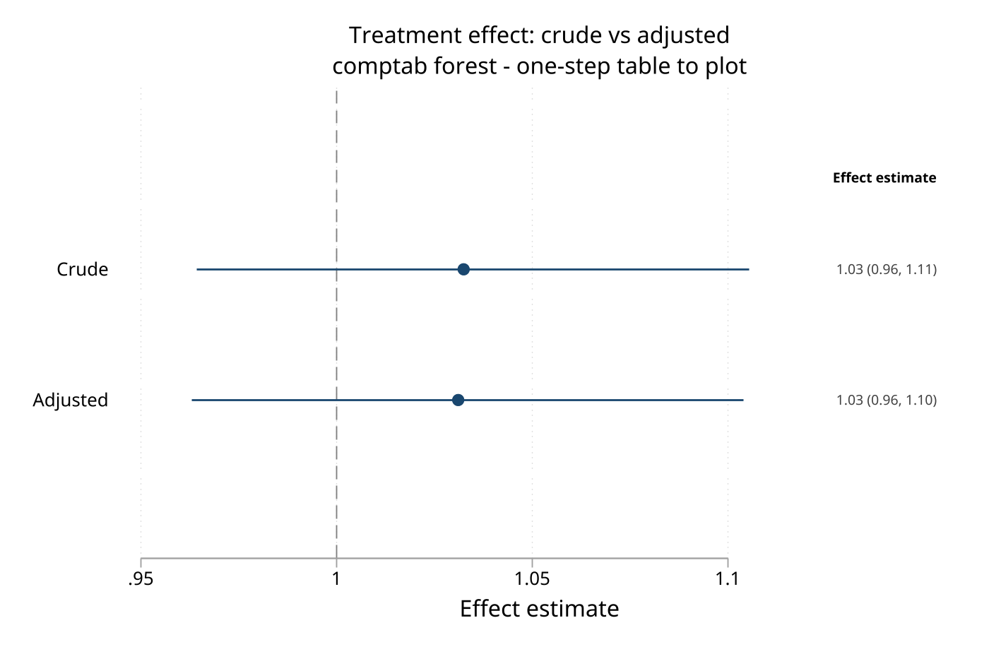
comptab and hrcomptab go one step further: their forest option composes companion frames from several models and calls eplot for you, passing graph options through eplotoptions().

comptab g_crude g_adj, rows(1 \ 1) section("Crude" \ "Adjusted") ///
    forest eplotoptions(null(1) title("Treatment effect: crude vs adjusted"))

The shared demo demo/demo_tabtools_eplot.do (also shipped in tabtools/demo/) builds both plots end to end from the bundled clinical cohort.

Option Reference

Options are organized by function. Not every option works in every mode — see help eplot for per-option mode availability.

Category	Options
Data specification	labels(), weights(), type()
Coefficient selection	keep(), drop(), rename(), noconstant
Labeling	coeflabels(), groups(), headers(), gap()
Transform	eform, rescale()
Reference lines	null(), nonull, xline(), xlabel()
Confidence intervals	level(), noci, cicap
Display	dp(), effect(), values, vformat(), stars, sigcolors, sigcolor(), insigncolor(), style(), favors()
Prediction/heterogeneity	pi(), i2(), tau2(), qstat()
Layout	horizontal, vertical, sort, order()
Multi-model	modellabels(), offset(), palette(), legendopts()
Markers	mcolor(), msymbol(), msize(), boxscale(), nobox, nodiamonds, cicolor(), ciwidth()
Graph	title(), subtitle(), note(), name(), saving(), scheme(), plotregion(), graphregion(), aspect(), plus any twoway option

Also See

• help eplot — full documentation with clickable examples
• coefplot (Ben Jann, SSC) — comprehensive coefficient plotting
• metan (SSC) — meta-analysis with forest plots
• Stata 18+: meta forestplot — official meta-analysis forest plots

Version History

• 1.2.0 (2026-06-06): Added frame input mode via eplot, frame(framename) with default estimate, ll, ul, label, rowtype, pvalue, and weight-variable detection for tabtools companion frames
• 1.1.1 (2026-04-30): Fixed y-axis ordering bug where categorical labels appeared in reverse order across all plotting modes (data, estimates, matrix)
• 1.1.0 (2026-04-19): Added gap() for grouped spacing, effect-axis xlabel() passthrough, automatic value-annotation margin sizing, and clearer mode-detection documentation
• 1.0.0 (2026-04-12): Initial release with data, estimates, and matrix modes; multi-model comparison; journal style presets; significance coloring; meta-analysis features

Author

Timothy P Copeland, Karolinska Institutet