finegray

Version 1.2.1 | 2026-08-11

finegray fits Fine-Gray subdistribution hazard models for a selected competing event in Stata 16 or later. The package also provides individual prediction, cumulative-incidence profiles and curves, proportional-hazards diagnostics, delayed-entry support, and optional bootstrap confidence intervals for cumulative-incidence quantities.

Quick Start

After installation, fit a model and request cumulative incidence at selected horizons:

webuse hypoxia, clear
gen byte status = failtype
stset dftime, failure(dfcens == 1) id(stnum)

finegray ifp tumsize pelnode, compete(status) cause(1)
finegray_cif, attime(1 5 8) ci

The selected event is cause(1) in status; status == 0 is treated as censored by default. The fitted model uses the declared stset analysis time and subject identifier.

Use finegray_predict for observation-level predictions and finegray_phtest for a proportional-hazards diagnostic:

finegray_predict double cif_hat, cif
finegray_phtest, time(log)

Requirements

• Stata 16 or later.
• Data declared with stset; an id() identifier is required, including when the data contain one record per subject.
• No external software or additional Stata package is required.

Installation

Install the released package from the Stata-Tools repository:

capture ado uninstall finegray
net install finegray, from("https://raw.githubusercontent.com/tpcopeland/Stata-Tools/main/finegray") replace

For a local checkout, replace the from() directory with the path to its finegray folder:

net install finegray, from("/path/to/Stata-Tools/finegray") replace

Commands

Command	Purpose
finegray	Fit a Fine-Gray subdistribution hazard model.
finegray_predict	Generate linear predictors, cumulative incidence, Schoenfeld residuals, or the baseline cumulative subdistribution hazard.
finegray_cif	Evaluate cumulative incidence at profiles or time points, optionally with confidence intervals or bootstrap confidence limits.
finegray_phtest	Inspect proportional-hazards behavior using raw Schoenfeld residual-time correlations.

How It Works

finegray estimates regression coefficients for the subdistribution hazard of the integer event value selected by cause() in the compete() variable. Competing events remain represented in the risk-set construction, while inverse-probability-of-censoring weights account for right censoring; the implementation uses a native Mata scan rather than expanding the data into pseudo-observations.

With a proportional subdistribution-hazards model, the exponentiated coefficient is a subdistribution hazard ratio (SHR), and the fitted baseline subdistribution hazard is combined with the linear predictor to obtain a cumulative-incidence function (CIF). The default display is exponentiated coefficients; use noshr for log-SHR coefficients.

The usual workflow is to declare survival-time data, fit one model, use finegray_predict for row-level quantities, use finegray_cif for a covariate profile or a curve, and use finegray_phtest to explore time-varying effects. xb can score compatible new data. Point cif and basecshazard predictions can also use compatible data while the active fit's cached event-time structure or a posted e(basehaz) is available; those quantities need _t or timevar(). finegray_cif, finegray_phtest, and the ci, schoenfeld, and bootstrap() paths of finegray_predict require the original, unchanged stset data.

For delayed entry, declare enter(time ...) in stset and fit with the package's Weight 1 risk-set construction. Use strata() for censoring groups and truncstrata() for entry groups; when both are specified, observed combinations form joint weighting groups. Inspect e(lt_weight), e(lt_vce), and the weight diagnostics before interpreting the result.

Choosing a Workflow

Goal	Command or pattern	Main considerations
Fit a model	finegray x1 x2, compete(status) cause(1)	Declare stset and id() first.
Score observations	finegray_predict newvar, xb	Compatible new data can be scored for the linear predictor.
Estimate row-level CIFs	finegray_predict newvar, cif timevar(t)	Use timevar() to evaluate all rows at a common horizon.
Compare a covariate profile	finegray_cif, at(...) attime(...)	at() supplies a profile; default profile values are estimation-sample means.
Draw a CIF curve	finegray_cif, timepoints(...)	Use ci, nograph, saving(), and twoway options as needed.
Explore proportional hazards	finegray_predict stub, schoenfeld; then finegray_phtest	The residual variables are optional for inspection; the diagnostic reports correlations, not an omnibus chi-squared test.
Account for delayed entry	stset ..., enter(time entry) plus finegray	Check positivity and the posted delayed-entry weight diagnostics.

Worked Examples

The examples below are intended to be run separately from a clean Stata session. Each uses Stata's webuse hypoxia example dataset.

1. Fit a basic model and inspect the estimates

webuse hypoxia, clear
gen byte status = failtype
stset dftime, failure(dfcens == 1) id(stnum)
finegray ifp tumsize pelnode, compete(status) cause(1)
ereturn list

2. Generate linear predictors and common-horizon CIFs

webuse hypoxia, clear
gen byte status = failtype
stset dftime, failure(dfcens == 1) id(stnum)
finegray ifp tumsize pelnode, compete(status) cause(1)
finegray_predict double xb_hat, xb
gen double horizon5 = 5
finegray_predict double cif5, cif timevar(horizon5) ci level(95)
summarize xb_hat cif5 cif5_lci cif5_uci

3. Estimate a profile-specific CIF table

webuse hypoxia, clear
gen byte status = failtype
stset dftime, failure(dfcens == 1) id(stnum)
finegray ifp tumsize pelnode, compete(status) cause(1)
finegray_cif, at(pelnode=1 ifp=20 tumsize=5) attime(1 3 5 8) ci
return list

4. Save a confidence-banded CIF curve on a custom grid

webuse hypoxia, clear
gen byte status = failtype
stset dftime, failure(dfcens == 1) id(stnum)
finegray ifp tumsize pelnode, compete(status) cause(1)
tempfile cifout
finegray_cif, timepoints(1 2 3 4 5 6 7 8) ci nograph saving("`cifout'", replace)
use "`cifout'", clear
list time cif se lci uci, noobs

5. Use factor variables and inspect proportional hazards

webuse hypoxia, clear
gen byte status = failtype
stset dftime, failure(dfcens == 1) id(stnum)
finegray i.pelnode c.ifp##c.tumsize, compete(status) cause(1)
finegray_predict double schoenfeld, schoenfeld
finegray_phtest, time(log) detail

6. Fit with censoring strata and clustered robust inference

webuse hypoxia, clear
gen byte status = failtype
gen int site = ceil(_n / 10)
stset dftime, failure(dfcens == 1) id(stnum)
finegray ifp tumsize pelnode, compete(status) cause(1) strata(pelnode) cluster(site)
display "clusters = " e(N_clust)

7. Use bootstrap confidence intervals for a CIF profile

webuse hypoxia, clear
gen byte status = failtype
gen int site = ceil(_n / 10)
stset dftime, failure(dfcens == 1) id(stnum)
finegray ifp tumsize pelnode, compete(status) cause(1) cluster(site)
finegray_cif, attime(1 5 8) ci bootstrap(25) seed(24680)
return list

The minimum is 25 replications; use substantially more replications for substantive inference.

8. Fit a delayed-entry model and inspect the weight path

webuse hypoxia, clear
gen byte status = failtype
gen double entry_time = dftime / 4
stset dftime, failure(dfcens == 1) id(stnum) enter(time entry_time)
finegray ifp tumsize pelnode, compete(status) cause(1)
display "weight method = " e(lt_weight)
display "weight VCE = " e(lt_vce)
finegray_cif, attime(3 5 8) ci

9. Request the baseline hazard and baseline cumulative subdistribution hazard

webuse hypoxia, clear
gen byte status = failtype
stset dftime, failure(dfcens == 1) id(stnum)
finegray ifp tumsize pelnode, compete(status) cause(1) basehaz
matrix list e(basehaz)
finegray_predict double baseline_subhaz, basecshazard
summarize baseline_subhaz

Demo

From the root of a Stata-Tools checkout, run the comprehensive demonstration:

stata-mp -b do finegray/demo/demo_finegray.do

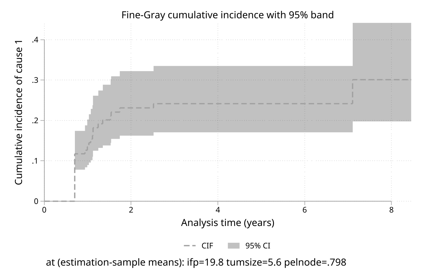
The script adds the local package directory to the session-only adopath, exercises fitting, prediction, diagnostics, CIF tables, delayed entry, string identifiers, bootstrap inference, and graph export, and regenerates demo/finegray_cif.png, shown below. A sibling tc_schemes checkout is optional for graph styling; the script falls back to Stata's s2color scheme.

The repository also includes demo/benchmark_finegray.do and demo/benchmark_large.do for optional timing comparisons.

The main demo regenerates this cumulative-incidence curve with a pointwise 95% confidence band:

Command Reference

finegray

finegray varlist [if] [in], compete(varname) cause(integer) [censvalue(integer) noshr level(#) strata(varlist) truncstrata(varlist) cluster(varname) norobust noadjust nolog basehaz nuisance iterate(integer) tolerance(#)]

finegray [, noshr level(#)]

The second form replays the last finegray results without refitting; noshr and level() are honored on replay.

varlist accepts numeric factor-variable notation, including continuous terms, indicators, interactions, and expanded interactions. compete() identifies the event-type variable and cause() selects the integer event value whose subdistribution hazard is modeled; censvalue() defaults to 0. The stset declaration supplies analysis time, failure coding, subject identifier, and optional delayed-entry time.

The default variance is a finite-sample-adjusted fixed-weight sandwich variance; with delayed entry, both censoring and entry weights are treated as fixed. The default display is the SHR scale. norobust requests the model-based inverse-information variance; noadjust suppresses the finite-sample sandwich adjustment and is available only with the robust variance. cluster() changes the sandwich clustering and strata() stratifies the right-censoring model.

truncstrata() is for delayed-entry risk-set weighting and requires delayed entry. nuisance adds the Fine-Gray right-censoring nuisance term to the sandwich variance and is not available for delayed entry. basehaz posts the optional baseline matrix needed for direct inspection. nolog, iterate(), and tolerance() control optimization output and convergence.

finegray_predict

finegray_predict [type] newvar [if] [in], [xb cif schoenfeld basecshazard timevar(varname) ci level(#) bootstrap(#) seed(#)]

An optional storage type such as double may precede newvar. The default is xb. cif generates cumulative incidence at each observation's _t, or at the numeric values in timevar(). ci adds newvar_lci and newvar_uci; confidence intervals require cif, and bootstrap intervals additionally require bootstrap() with at least 25 replications. seed() requires bootstrap().

schoenfeld generates a stub for the raw Schoenfeld residuals, followed by numbered variables for additional model terms. basecshazard generates the fitted baseline cumulative subdistribution hazard and cannot be combined with ci or bootstrap(). The prediction types are mutually exclusive.

finegray_cif

finegray_cif [, at(string) attime(numlist) timepoints(numlist) ci level(#) saving(filename[, replace]) bootstrap(#) seed(#) nograph twoway_options]

Use at() to define a covariate profile; unspecified covariates default to estimation-sample means. Use attime() for a table at requested horizons or timepoints() for a curve grid; the two options are mutually exclusive. With neither option, the command uses the distinct baseline event-time grid, thinned when necessary.

ci requests pointwise confidence limits, nograph suppresses the graph, and saving() writes time, cif, se, lci, and uci to a Stata dataset. bootstrap() refits the model for at least 25 subject- or cluster-level replications; seed() requires bootstrap(). Remaining options are passed to the underlying twoway graph. In attime() mode, graph options are ignored with a note.

finegray_phtest

finegray_phtest [, time(function) detail]

The default time(rank) scale uses event-time ranks; time(log) uses log event time and time(identity) uses event time. The command reports term-level correlations between raw Schoenfeld residuals and the selected time scale, along with event counts. detail displays the first 20 event-level residual contributions. This is an exploratory diagnostic and does not post an omnibus chi-squared statistic or p-value.

Options

Estimation options

Option	Default and use
compete(varname)	Required event-type variable; it must agree with the stset failure coding.
cause(#)	Required integer event code to model; it must differ from censvalue().
censvalue(#)	0; value treated as right censoring in compete().
strata(varlist)	None; stratifies the right-censoring model.
truncstrata(varlist)	None; delayed-entry truncation strata for Weight 1 estimation.
cluster(varname)	None; cluster variable for the sandwich variance.
norobust	Off; use model-based rather than sandwich variance.
noadjust	Off; suppress the finite-sample sandwich adjustment.
noshr	Off; display log-SHR coefficients instead of exponentiated coefficients.
level(#)	c(level); confidence level from 10 to below 100 for displayed intervals and postestimation.
nolog	Off; suppress the iteration log.
basehaz	Off; post the baseline cumulative subdistribution hazard in e(basehaz).
nuisance	Off; add the right-censoring nuisance term to the sandwich variance. Not available with delayed entry.
iterate(#)	200; maximum number of optimization iterations.
tolerance(#)	1e-8; convergence tolerance.

norobust, noadjust, and nuisance have compatibility restrictions documented in the command help. In particular, noadjust is meaningful only with the sandwich variance, and the model-based path cannot be combined with cluster().

Prediction options

Option	Use
xb	Generate the linear predictor; this is the default prediction type.
cif	Generate cumulative incidence at _t or at timevar().
schoenfeld	Generate raw Schoenfeld residual variables on the original estimation data.
basecshazard	Generate the baseline cumulative subdistribution hazard.
timevar(varname)	Numeric evaluation time for cif or basecshazard.
ci	Add lower- and upper-confidence-limit variables for cif.
level(#)	c(level); confidence level from 10 to below 100 for ci.
bootstrap(#)	At least 25 refits for bootstrap CIF confidence limits.
seed(#)	Reproducible bootstrap seed; requires bootstrap().

CIF and diagnostic options

Option	Use
at(string)	Profile values for finegray_cif; unspecified covariates use estimation-sample means.
attime(numlist)	Fixed horizons for a returned CIF table.
timepoints(numlist)	Evaluation grid for a returned CIF curve.
saving(filename[, replace])	Save CIF curve data with time, cif, se, lci, and uci.
nograph	Suppress the CIF graph.
twoway_options	Graph options passed to the CIF twoway graph.
time(function)	Time scale for finegray_phtest: rank, log, or identity; default rank.
detail	Show the first 20 event-level diagnostic contributions.

For finegray_cif, attime() and timepoints() cannot be combined. ci uses pointwise influence-function limits; bootstrap() uses refitted subject- or cluster-level samples and can report requested, successful, and failed replications in r().

Stored Results

After finegray

Standard estimation results include e(b), e(V), e(sample), e(N), e(depvar), and e(properties). e(depvar) is _t, the stset analysis time, as it is after stcrreg; the event-type variable is e(compete). For a factor-variable fit, e(b) and e(V) are named with the terms you typed (1.pelnode, 1.pelnode#c.ifp), so test, testparm, and estimates table address them directly; the internal design columns are listed in e(covariates). The command also posts these scalars (with e(N_clust) when clustering is used):

e(N_fail), e(N_compete), e(N_cens), e(ll), e(ll_0), e(chi2), e(p), e(df_m), e(rank), e(N_clust), e(converged), e(N_delayed), e(N_G_trunc), e(level), e(cause), e(censvalue), e(iterate), e(tolerance), e(N_weight_strata), e(min_weight_prob), e(max_lt_weight), e(N_prob_warn), and e(N_weight_warn).

Posted macros are e(cmd), e(cmdline), e(refitcmd), e(predict), e(compete), e(compete_values), e(covariates), e(fvvarlist), e(fvsemantic), e(strata), e(truncstrata), e(clustvar), e(lt_weight), e(lt_vce), e(bh_seq), e(weight_warn_strata), e(vce), e(vce_meat), e(title), e(marginsok), e(datasignature), and e(datasignaturevars).

The optional matrix e(basehaz) has columns for event time and cumulative baseline subdistribution hazard and is posted only when basehaz is specified. e(N_clust) is posted when clustering is used; delayed-entry diagnostics are populated when delayed-entry weighting applies.

After finegray_cif

The returned matrix r(table) contains the CIF table or curve, and r(at) contains the evaluated profile. Scalars are r(level) and r(cause). With bootstrap(), the command additionally posts r(bootstrap_requested), r(bootstrap_success), and r(bootstrap_failed); r(profile_vars) identifies the profile variables used.

After finegray_phtest

The command posts r(N_fail), r(time), r(residual_scale), and matrix r(phtest). The matrix contains term-level correlations and event counts; no omnibus chi-squared result is posted.

After finegray_predict

finegray_predict clears r() and does not post estimation results. It creates the requested variable, plus _lci and _uci variables for cif, ci, or numbered Schoenfeld-residual variables when the requested stub represents multiple model terms.

Assumptions and Limits

• stset must define the analysis time, failure indicator, and id(); finegray rejects an empty analysis sample and inconsistent competing-event coding.
• Multiple records per subject are supported when intervals are contiguous and covariates, censoring strata, truncation strata, and cluster membership are constant within subject. The estimation sample is reduced to one subject-level record for the fitted model, while interval records remain available for relevant postestimation quantities.
• Time-varying covariates, by prefixes, fweights, and pweights are not supported. Factor variables and interactions are supported, but a scoring dataset must contain compatible values and factor levels.
• The default variance treats estimated censoring weights as fixed and, with delayed entry, also treats entry weights as fixed; it uses a sandwich estimator. norobust requests model-based information-matrix variance and is not a general replacement when weights are estimated.
• nuisance is limited to right-censoring models, adds the nuisance term to the sandwich variance, and cannot be combined with delayed-entry weighting. The default delayed-entry variance is fixed-weight; coefficient inference that includes weight-estimation variability requires bootstrapping the whole fit externally.
• Delayed entry uses the package's Weight 1 construction. It checks censoring/truncation positivity and observed grouping support; weights can exceed 1. strata() defines censoring groups and truncstrata() defines entry groups; observed combinations form joint weight strata, with at most 100 cells and at least 20 estimation-sample subjects per cell. Continuous covariate-dependent entry is not supported.
• Postestimation requires a converged fit. finegray_cif, finegray_phtest, and the ci, schoenfeld, and bootstrap() paths of finegray_predict require the original, unchanged stset data. Point xb predictions work on compatible new data; point cif and basecshazard predictions can also do so while the active fit has its cached or posted baseline. Package-created factor-design columns may be dropped and rebuilt on demand, but retain _fg_entry for postestimation after a multiple-record fit; modifying a present _fg_* design column in place is rejected.
• finegray_phtest is a residual-correlation diagnostic rather than a formal omnibus test. Interpret it alongside the scientific model and the observed event-time support.

References

• Fine JP and Gray RJ (1999). A proportional hazards model for the subdistribution of a competing risk. Journal of the American Statistical Association, 94(446), 496–509. doi:10.1080/01621459.1999.10474144.
• Zhang X, Zhang M-J, and Fine J (2011). A proportional hazards regression model for the subdistribution with right-censored and left-truncated competing risks data. Statistics in Medicine, 30(16), 1933–1951. doi:10.1002/sim.4264.
• Geskus RB (2011). Cause-specific cumulative incidence estimation and the Fine and Gray model under both left truncation and right censoring. Biometrics, 67(1), 39–49. doi:10.1111/j.1541-0420.2010.01420.x.
• Bellach A, Kosorok MR, Gilbert PB, and Fine JP (2020). General regression model for the subdistribution of a competing risk under left-truncation and right-censoring. Biometrika, 107(4), 949–964. doi:10.1093/biomet/asaa034.
• Kawaguchi ES, Shen JI, Suchard MA, and Li G (2021). Scalable algorithms for large competing risks data. Journal of Computational and Graphical Statistics, 30(3), 685–693. doi:10.1080/10618600.2020.1841650.
• Li J, Scheike TH, and Zhang MJ (2015). Checking Fine and Gray subdistribution hazards model with cumulative sums of residuals. Lifetime Data Analysis, 21(2), 197–217. doi:10.1007/s10985-014-9313-9.

QA

QA suites and how to run them are documented in qa/README.md.

Version History

• 1.2.1 (2026-08-11): Fixed cold-cache CIF and baseline-hazard prediction after multiple-record reduction, prediction with legal long factor-variable names, confidence-level validation in both CIF commands, and a false delayed-entry positivity error for competing exits after the last cause event.
• 1.2.0 (2026-08-10): Added delayed-entry Weight 1 paths, robust-variance adjustment controls, nuisance-adjusted sandwich inference, optional baseline-hazard output, and expanded CIF and diagnostic workflows; finegray_phtest is an exploratory residual-correlation diagnostic without an omnibus test. Display and reporting pass: finegray now replays its results when typed with no varlist; factor-variable coefficients are named with the terms you typed rather than internal design columns (so test 1.pelnode and estimates table work directly); the header reports the competing event values, the delayed-entry weight and late-entry count, and which variance is in e(V); e(depvar) is _t, matching stcrreg. finegray_cif states the covariate profile above the table and under the graph, extends the plotted curve across the flat tail to the end of follow-up, flags requested times outside the estimated support, and labels the saving() dataset. New returns: e(N_delayed), e(N_G_trunc), e(compete_values). Documentation and diagnostics pass: the factor-variable naming guidance now matches the user-facing coefficient names stored in e(b) and e(V); ibn. is documented as estimable inside an interaction but refused as a main effect, with the refusal naming the terms you typed rather than internal design columns; the margins limitation is stated precisely (factor terms give r(322), continuous-covariate margins remain valid); post-estimation on an empty e(sample) — what estimates use leaves behind — now reports that rather than "data have changed", and the help explains how estimates esample: restores it; rendered help spacing repaired throughout and the option tables fit an 80-column Viewer.
• 1.1.0 (2026-07-10): Added CIF curves, multiple-record support, stratified censoring, and postestimation confidence intervals.
• 1.0.0 (2026-04-06): Initial Stata-Tools release of finegray, finegray_predict, and finegray_phtest.

Author

Timothy P Copeland, Karolinska Institutet

License

MIT