iivw
AnalysisInverse intensity of visit weighting (IIW, IPTW, FIPTIW) for irregular longitudinal data
Version 1.5.1 | 2026-06-11
iivw corrects bias from informative visit timing in irregular longitudinal data and provides diagnostics for separating sampling bias from residual measurement artifact. In clinic-based studies, sicker patients often visit more frequently, so they contribute more rows to the dataset and bias naive analyses. This package re-weights each observation so the fitted outcome model targets the patient population more directly rather than the clinic-visit process.
Three weighting strategies are available:
- IIW (inverse intensity weighting) — corrects for outcome-dependent visit frequency
- IPTW (inverse probability of treatment weighting) — corrects for confounding by treatment indication
- FIPTIW (IIW × IPTW) — corrects for both simultaneously
Outcome models are fit via GEE-style estimation (GLM with clustered robust SEs) or mixed effects, either unweighted or with IIW/IPTW/FIPTIW weights.
Requirements
- Stata 16 or later
- Stata 17 or later for
iivw_fit, model(mixed) - Optional:
tabtoolsfor theregtabmodel-table Excel examples
Installation
capture ado uninstall iivw
net install iivw, from("https://raw.githubusercontent.com/tpcopeland/Stata-Tools/main/iivw") replace
Commands
| Command | Description |
|---|---|
iivw |
Package overview and available commands |
iivw_weight |
Compute IIW, IPTW, or FIPTIW weights |
iivw_balance |
Check weight leverage and visit-model balance |
iivw_fit |
Fit weighted or unweighted outcome models through a consistent interface |
iivw_exogtest |
Check whether lagged outcome/disease activity predicts future visit timing |
iivw_diagnose |
Compare unweighted, weighted, and artifact-adjusted marginal/reference-slope estimates |
Plain-Language Summary
Longitudinal clinic data usually has one row per visit. If some patients visit more often because they are getting worse, those patients also appear more often in the dataset. A standard regression then partly answers the wrong question: it estimates an association in the visit process, not only in the patient population.
iivw estimates how likely each observed visit was, then gives less influence to visits that were very likely to occur and more influence to visits that were less likely to occur. If treatment assignment is also confounded, iivw can multiply those visit weights by propensity-score treatment weights.
Use the package as a weighting workflow:
iivw_weightcreates weights and stores the panel metadata.iivw_balancechecks whether those weights have enough leverage and a usable visit-model balance profile.iivw_fitreads those weights and fits the weighted outcome model.
When Do I Need This?
You likely need this package if:
- Your data comes from a clinical registry, electronic health records, or any setting where visit times are determined by clinical need rather than a fixed protocol.
- You have longitudinal data with unequal numbers of visits per subject, and sicker (or healthier) patients are observed more often.
- You want to estimate a treatment effect, disease trajectory, or covariate association and need to remove bias from informative visit timing.
You probably do not need this if visits follow a fixed protocol (e.g., randomized trial with scheduled assessments) or if the main concern is dropout rather than differential visit frequency.
How It Works
- Compute weights with
iivw_weight. You always specifyid()andtime(). For IIW/FIPTIW, the command fits an Andersen-Gill recurrent-event Cox model to estimate each subject's visit intensity; for IPTW-only, it fits only the treatment propensity model. It then creates a weight variable in the dataset. - Choose the weighting strategy that matches the scientific problem (see table below).
- Inspect diagnostics with
iivw_balancefor the visit-intensity model. Whentreat()andtreat_cov()are used, runpsdash combinedfor treatment-propensity overlap, common support, balance, and treatment-weight diagnostics. - Fit the outcome model with
iivw_fit. It reads the weight variable and panel structure from the dataset automatically.
Recommended Analysis Recipes
Use these as starting templates, then adapt the covariates to the study design.
Descriptive disease trajectory in registry data
Goal: estimate a population-average longitudinal trajectory when sicker patients are seen more often.
iivw_weight, id(id) time(months) ///
    visit_cov(age sex baseline_score baseline_edss clinic_year) ///
    lagvars(current_score relapse) truncate(1 99) efron nolog

iivw_fit current_score age sex baseline_score, ///
    timespec(ns(3)) nolog
Report the visit model, the weight distribution, effective sample size, and whether the trajectory changes materially when using timespec(linear) instead of timespec(ns(3)).
Binary treatment comparison with informative visits
Goal: compare treatment groups when both treatment assignment and follow-up frequency depend on baseline severity.
iivw_weight, id(id) time(months) ///
    visit_cov(age sex baseline_edss baseline_score clinic_year) ///
    lagvars(current_score relapse) ///
    treat(treated) treat_cov(age sex baseline_edss baseline_score) ///
    truncate(1 99) efron replace nolog

psdash combined, saving(treatment_ps_dashboard.png)
psdash weights, iivwcomponent(final) graph saving(final_fiptiw_weight.png)
iivw_balance, agrefit nolog

iivw_fit current_score treated age sex baseline_score, ///
    timespec(linear) nolog
Use this only when treated is a binary, time-invariant subject-level exposure. If treatment switches during follow-up, this package is not a substitute for a time-varying treatment MSM.
Time-varying treatment effect or treatment trajectory
Goal: test whether the treatment contrast changes as follow-up accumulates.
iivw_fit current_score treated age sex baseline_score, ///
    timespec(ns(3)) interaction(treated) replace nolog
Interpret the interaction terms as a sensitivity description unless the time scale and functional form were prespecified. For a single clinically interpretable contrast at a time point, use Stata post-estimation tools such as margins or lincom after iivw_fit.
Sampling bias versus measurement artifact
Goal: compare movement from weighting against movement from direct adjustment for repeated measurement, test practice, or cumulative testing.
Use the detailed diagnostic workflow below. The main decomposition target should be a marginal or reference-arm time slope, not the treatment-by-time contrast.
Diagnostic Workflow: Sampling Bias vs Measurement Artifact
IIVW corrects bias from the observation process. It cannot remove bias that lives inside the measurement itself, such as practice effects from repeated cognitive testing. The diagnostic workflow compares how much the marginal/reference-arm time slope moves after weighting and how much it moves after direct adjustment for the measurement process.
* 1. Unweighted model through the same outcome-model interface
iivw_fit sdmt_score treatment months_since_tx interaction age sex, ///
    unweighted id(id) time(months_since_tx) timespec(none) nolog
estimates store M_unweighted

* 2. FIPTIW weighted model
iivw_weight, id(id) time(months_since_tx) ///
    visit_cov(treatment age sex bl_edss bl_sdmt) ///
    lagvars(sdmt_score recent_relapse) ///
    treat(treatment) treat_cov(age sex bl_edss bl_sdmt) ///
    truncate(1 99) efron replace nolog

iivw_balance, nolog

iivw_fit sdmt_score treatment months_since_tx interaction age sex, ///
    timespec(none) nolog
estimates store M_weighted

* 3. Measurement-process adjustment
gen double log_test_number = log(test_number + 1)
iivw_fit sdmt_score treatment months_since_tx interaction age sex log_test_number, ///
    timespec(none) replace nolog
estimates store M_adjusted

* 4. Check exogeneity of testing schedule
iivw_exogtest sdmt_score recent_relapse, ///
    id(id) time(months_since_tx) adjust(age sex bl_edss bl_sdmt) ///
    by(treatment) efron nolog

* 5. Check whether a null weighting movement is informative
iivw_balance, nolog

* 6. Quantify diagnostic movement
iivw_diagnose months_since_tx, ///
    unweighted(M_unweighted) weighted(M_weighted) adjusted(M_adjusted) ///
    exogeneity(unknown)
The decomposition target is the marginal or reference-arm time slope. A large unweighted-to-weighted movement suggests sampling bias. A small weighting movement but large measurement-adjustment movement suggests residual measurement artifact. Treatment x time contrasts can be reported as ordinary sensitivity estimates, but they should not be interpreted with the sampling/artifact share formula. If iivw_exogtest finds lagged outcome predictors of visit timing, the measurement-process adjustment may be endogenous and should be read as a bound or sensitivity result rather than a clean correction.
iivw_balance returns r(informative), a single workflow flag that is 1 only when weight leverage is not low and the modeled visit-covariate balance flag is good. iivw_diagnose returns point diagnostic quantities. It does not produce an interval for the artifact share; that requires a subject-level bootstrap that refits all three models together.
Diagnostic Decision Guide
| Pattern | Practical interpretation | Reporting language |
|---|---|---|
| Large unweighted-to-weighted movement, small measurement-adjustment movement | The visit process likely explains much of the naive trajectory distortion | "Results were sensitive to IIVW/FIPTIW correction, suggesting informative visit timing." |
| Small weighting movement, large measurement-adjustment movement | Repeated measurement or practice/test artifact may dominate | "Direct measurement-process adjustment changed the marginal slope more than weighting." |
iivw_exogtest p-values small |
Lagged outcomes predict future testing or visits; direct adjustment may be endogenous | "The adjusted estimate is presented as a sensitivity bound rather than a clean correction." |
| Total gap near zero | Share estimates are unstable because there is little movement to decompose | "The three estimates were similar; artifact shares are not informative." |
| Sampling or artifact shares outside 0 to 1 | Model movement is sign-inconsistent | "The decomposition is descriptive and sign-inconsistent; focus on the three estimates." |
For expert analyses, the diagnostic workflow is best treated as a structured sensitivity analysis. The package helps make the comparison reproducible, but the scientific claim still depends on whether the visit model, treatment model, and measurement-process adjustment are credible for the design.
Choosing a Weight Type
| Weight type | When to use | Key iivw_weight options |
|---|---|---|
iivw |
Visit timing is informative, but treatment weighting is not needed | id() time() visit_cov() |
iptw |
Treatment confounding only (visits are protocol-driven) | treat() treat_cov() wtype(iptw) |
fiptiw |
Both informative visit timing and treatment confounding | id() time() visit_cov() treat() treat_cov() |
By default, iivw_weight auto-detects the type: specifying treat() triggers FIPTIW; omitting it triggers IIW. Override with wtype().
Data Contract
iivw_weight expects long panel data: one row per subject-visit. id() identifies the subject, and time() identifies visit time. The id() and time() combination must be unique and nonmissing. For IIW and FIPTIW, each subject needs at least two visits because the command estimates a visit-intensity model from inter-visit intervals.
For IPTW and FIPTIW, treat() must be a binary 0/1 treatment indicator, observed on every row, and constant within subject. Treatment-model covariates are supplied with treat_cov() and are not inferred from visit_cov(). IPTW-only analyses can use one row per subject by specifying wtype(iptw).
What Gets Added to the Data
By default, iivw_weight creates _iivw_weight, the final weight used by iivw_fit. It also creates component variables when needed: _iivw_iw for visit-intensity weights, _iivw_ps for the treatment propensity score, and _iivw_tw for treatment weights. Use generate(prefix) to change the prefix.
The weighting step also stores dataset metadata, including the panel ID, time variable, weight type, weight variable, component variables, prefix, expanded visit-model covariate list, treatment variable, treatment-model covariates, and the treatment propensity-score contract. iivw_balance, iivw_fit, and psdash read that metadata automatically, so the usual workflow is to run iivw_weight, inspect the relevant diagnostics, and then run iivw_fit without re-entering the panel structure.
Using psdash with iivw
When iivw_weight is run with treat() and treat_cov(), the treatment propensity model can be diagnosed with psdash.
Run psdash combined immediately after iivw_weight to inspect treatment-propensity overlap, common support, treatment-covariate balance, and treatment-weight distribution. Then run iivw_balance for the visit-intensity component. The two diagnostics answer different questions: psdash checks treatment positivity and treatment-model balance; iivw_balance checks whether visit-intensity weights have enough leverage and whether modeled visit covariates are balanced.
iivw_weight, id(id) time(months) ///
    visit_cov(age sex bl_edss bl_sdmt) ///
    lagvars(sdmt relapse) ///
    treat(treated) treat_cov(age sex bl_edss bl_sdmt) ///
    truncate(1 99) efron replace nolog

psdash combined, saving(treatment_ps_dashboard.png)
psdash weights, iivwcomponent(final) graph saving(final_fiptiw_weight.png)
iivw_balance, agrefit nolog
iivw_fit sdmt treated age sex bl_edss, timespec(ns(3)) nolog
Choosing Covariates
The most common practical mistake is treating visit_cov() and treat_cov() as interchangeable lists. They answer different design questions.
| Covariate role | Put it in | Rationale |
|---|---|---|
| Baseline disease severity that drives both visits and treatment | visit_cov() and treat_cov() |
It can confound both observation and treatment assignment |
| Previous outcome value or recent event | lagvars() or a precomputed lag in visit_cov() |
It predicts future visit intensity without using the current visit outcome to explain itself |
| Demographic or calendar design variable | Usually both models if it affects both mechanisms | It can capture structural visit access and treatment patterns |
| Post-treatment mediator | Usually neither treatment model nor primary outcome covariate unless explicitly planned | It can change the estimand if adjusted for casually |
| Cumulative test count or practice-effect proxy | Outcome model diagnostic adjustment, not visit_cov() by default |
It is part of the measurement process being evaluated |
Start with a subject-matter model that is smaller than the full dataset dictionary. Add variables because they plausibly drive the visit or treatment process, not because they improve in-sample fit. If the final weights are extreme or ESS is poor, simplify before interpreting a highly variable weighted estimate.
Assumptions and Limits
The weights are a tool for a specific bias problem. They do not make a weak study design causal by themselves.
| Requirement | Why it matters |
|---|---|
| Visit model covariates capture the drivers of visit timing | IIW only removes bias explained by measured covariates |
| Treatment model covariates capture measured treatment confounding | IPTW/FIPTIW assume no unmeasured confounding after adjustment |
| Treatment is binary and time-invariant within subject | Current IPTW/FIPTIW implementation is not for treatment switching |
| Positivity/overlap is plausible | Subjects with near-certain treatment or visits create extreme weights |
| Outcome model includes the scientific predictors of interest | Weights correct sampling/visit imbalance; they do not choose the outcome model |
| Standard errors treat weights as fixed | Built-in sandwich and bootstrap SEs do not re-estimate weights |
For dropout or censoring, use an IPCW strategy. For time-varying treatment decisions, use a marginal structural model designed for that setting.
Worked Examples
These examples use a self-contained synthetic panel because Stata does not ship a built-in irregular-visit dataset that exercises the full workflow.
1. Create example longitudinal data
This creates 80 subjects with 4 visits each, a continuous disability outcome (EDSS), a binary treatment, and a binary event (relapse) that also predicts visit frequency.
clear
set seed 20260417
set obs 320
gen long id = ceil(_n/4)
bysort id: gen byte visit = _n
gen double days = (visit - 1) * 90 + runiform() * 20
replace days = 0 if visit == 1
gen double edss_bl = 2 + 3 * runiform()
bysort id: replace edss_bl = edss_bl[1]
gen double age = 35 + 15 * runiform()
bysort id: replace age = age[1]
gen byte sex = runiform() > 0.5
bysort id: replace sex = sex[1]
gen byte treated = (runiform() < invlogit(-0.8 + 0.5 * edss_bl))
bysort id: replace treated = treated[1]
gen double edss = edss_bl + 0.012 * days - 0.7 * treated + rnormal(0, 0.45)
gen byte relapse = (runiform() < invlogit(-2 + 0.4 * edss))
gen byte treatment = cond(treated == 0, 0, cond(edss_bl < 3.5, 1, 2))
label define arm 0 "Placebo" 1 "Low dose" 2 "High dose"
label values treatment arm
2. IIW only: correct the visit process
When the main concern is that patients with worse disease are seen more often, but treatment assignment is either randomized or not being analyzed:
iivw_weight, id(id) time(days) ///
    visit_cov(edss_bl age sex) lagvars(edss relapse) nolog
iivw_balance
summarize _iivw_weight, detail
iivw_fit edss treated edss_bl, model(gee) timespec(linear)
After computing weights, always inspect the distribution before fitting the outcome model. If the weight tails are extreme (e.g., max > 10), re-run iivw_weight with truncate(1 99). For real analyses, prefer baseline or lagged time-varying predictors in the visit model when the current visit measurement should not be used to explain the timing of that same visit.
3. FIPTIW: correct visit timing and treatment confounding together
Add treat() and treat_cov() when treatment assignment is also non-random:
iivw_weight, id(id) time(days) ///
    visit_cov(edss_bl age sex) lagvars(edss relapse) ///
    treat(treated) treat_cov(age sex edss_bl) ///
    truncate(1 99) replace nolog

iivw_fit edss treated age sex edss_bl, model(gee) timespec(quadratic)
4. Add time-varying effects in the weighted outcome model
Once weights are in place, iivw_fit can add flexible time trends and time × covariate interactions:
iivw_fit edss treated age sex edss_bl, ///
    model(gee) timespec(ns(3)) interaction(treated) replace
Use timespec(linear), timespec(quadratic), timespec(cubic), timespec(ns(#)), timespec(categorical), or timespec(none) depending on how flexible the time trend should be. Start with linear, then compare to ns(3) to check sensitivity. Use categorical when time is a small set of meaningful visit waves or calendar periods.
5. Use categorical predictors in the outcome model
categorical() expands a multi-level variable into labeled dummy variables. It affects the outcome model only — it does not create multi-arm IPTW.
iivw_weight, id(id) time(days) ///
    visit_cov(edss_bl age sex) lagvars(edss relapse) replace nolog
iivw_fit edss treatment edss_bl, ///
    categorical(treatment) timespec(ns(3)) interaction(treatment) replace
6. Use categorical time for visit-wave effects
timespec(categorical) expands the stored time variable into labeled non-reference time indicators. Use value labels on the time variable so collect and regtab get readable rows.
label define wave 1 "Baseline" 2 "Month 6" 3 "Month 12", replace
label values visit_wave wave

iivw_weight, id(id) time(visit_wave) ///
    visit_cov(edss_bl relapse) replace nolog
iivw_fit edss treatment edss_bl, ///
    timespec(categorical) timebasecat(1) ///
    categorical(treatment) interaction(treatment) replace collect
regtab, xlsx(iivw_results.xlsx) sheet(Waves) title(Treatment by Visit Wave)
Generated coefficient names stay short and predictable, such as _iivw_tcat_1 and _iivw_ix_drug_tcat_1, while variable labels carry table-ready text such as Visit wave: Month 6 (vs. Baseline) and Drug x Visit wave: Month 6. Use the generated names for post-estimation commands and the labels for exported tables.
7. Bootstrap standard errors
Bootstrap replicates apply to the outcome model fit with fixed weights. The weights are not re-estimated inside each bootstrap draw. Bootstrap clustering uses cluster() when specified and otherwise defaults to the subject ID stored by iivw_weight:
iivw_fit edss treated edss_bl, bootstrap(500) nolog replace
8. Export results to Excel
Use the collect option with non-bootstrap model(gee) fits and regtab (from the tabtools package) to build publication-ready model tables:
collect clear
iivw_fit edss treated edss_bl, model(gee) nolog replace collect
regtab, xlsx(iivw_results.xlsx) sheet(Results) title(IIW Analysis) stats(n)
iivw_balance, iivw_exogtest, and iivw_diagnose can also export their diagnostic tables directly, without requiring tabtools:
iivw_balance, xlsx(iivw_results.xlsx) sheet(Balance) replace

iivw_exogtest sdmt_score recent_relapse, ///
    id(id) time(months_since_tx) adjust(age sex bl_edss bl_sdmt) ///
    by(treatment) efron nolog xlsx(iivw_results.xlsx) sheet(Exogeneity)

iivw_diagnose months_since_tx, ///
    unweighted(M_unweighted) weighted(M_weighted) adjusted(M_adjusted) ///
    exogeneity(unknown) xlsx(iivw_results.xlsx) sheet(Diagnostics) replace
These direct exports are workbook-only: each command writes a styled .xlsx sheet with tabtools/regtab-style title, group-header, statistic-header, label-column, border, width, and footnote conventions. Existing workbooks are updated by replacing only the named sheet. iivw_balance and iivw_exogtest use variable-label row headers when labels are available. For iivw_exogtest, replace still means overwrite generated lag variables, not Excel workbook replacement.
Weight Diagnostics
After running iivw_weight, check these before fitting the outcome model:
| Diagnostic | What to look for | Action if concerning |
|---|---|---|
iivw_balance |
r(leverage) == "low" or r(informative) == 0 |
Treat null weighting movement as uninformative; revisit visit model |
summarize _iivw_weight, detail |
Max > 10, max/min ratio > 100 | Add truncate(1 99) |
| Effective sample size (reported automatically) | ESS much less than N | Simplify the visit model or truncate |
| Weight mean (reported automatically) | Mean far from 1.0 | Check model specification |
| Compare with/without truncation | Treatment effect changes substantially | Result may be driven by a few extreme weights |
psdash combined (IPTW/FIPTIW only) |
Poor treatment PS overlap, common-support loss, or residual treatment-covariate imbalance | Revisit treat_cov() and treatment positivity |
psdash weights, iivwcomponent(final) detail graph |
Extreme final FIPTIW/IPTW analysis weights | Check both treatment and visit components; consider truncation |
Common Problems and Fixes
| Symptom | Likely cause | Fix |
|---|---|---|
treat() contains missing values |
Treatment is missing on one or more visit rows | Fill the baseline treatment consistently within subject, or exclude those subjects deliberately |
treat() must be time-invariant |
Treatment changes over time | Do not use this IPTW/FIPTIW implementation; use a time-varying treatment/MSM approach |
requires at least 2 visits per subject |
IIW/FIPTIW needs repeated visits | Use repeated-visit data, or use wtype(iptw) for treatment weighting only |
| Very large weights | Sparse overlap, overfit model, or unusual visit patterns | Inspect covariates, simplify the model, and try truncate(1 99) |
variable ... already exists |
Re-running created-variable steps | Add replace if overwriting is intended |
iivw_fit says weights are missing |
Dataset changed or weights were dropped after iivw_weight |
Re-run iivw_weight immediately before iivw_fit |
Interpreting Results
- Coefficients (default GEE with gaussian family) are the change in the outcome per one-unit change in the predictor, averaged over the population.
- Treatment effect: The coefficient on the treatment variable is the weighted treatment contrast. A causal interpretation additionally requires a correctly specified visit model, a correctly specified propensity model for IPTW/FIPTIW, no unmeasured confounding, and a treatment assignment mechanism appropriate for the chosen weight type.
- Standard errors are sandwich (robust) SEs clustered at
cluster()when specified and otherwise at the subject ID stored byiivw_weight. They do not account for weight estimation uncertainty. - Post-estimation: All standard Stata post-estimation commands work after
iivw_fit(predict,lincom,test,margins).
What to Report
For technical reports and papers, include enough detail for readers to assess the weighting step:
- weight type used (
iivw,iptw, orfiptiw) - visit model covariates and whether
efrontie handling was used - treatment model covariates for IPTW/FIPTIW
- whether weights were stabilized with
stabcov()and/or truncated withtruncate() - weight diagnostics: mean, min, max, selected percentiles, and effective sample size
iivw_balanceleverage, balance flag, andr(informative)result- outcome model family/link, time specification, clustering level, and whether SEs were sandwich or bootstrap
- unweighted, weighted, and measurement-adjusted estimates for the marginal/reference time-slope coefficient when using the diagnostic workflow
- the
iivw_exogtestspecification and whether lagged outcome or disease-activity variables predicted visit timing - the
iivw_diagnosesampling/artifact gaps or endogenous diagnostic range - the definition of the measurement-process adjustment, such as raw cumulative test count,
log(test+1), inter-test interval, or categorical test occasion
Practical Notes
treat()must be observed on every row used in IPTW/FIPTIW, binary (0/1), and time-invariant within each subject. For time-varying treatments, consider marginal structural models instead.treat_cov()is required for IPTW and FIPTIW; treatment-model covariates are not inferred fromvisit_cov().- IPTW-only analyses may use one row per subject. IIW and FIPTIW require repeated visits because they estimate a visit-intensity model.
iivw_balanceautomatically reads the stored visit-model covariates fromiivw_weight; reruniivw_weightif older datasets do not contain that metadata.iivw_fitautomatically reads the weight variable, panel ID, and time variable stored byiivw_weight.iivw_fit, unweightedcan fit the same outcome-model surface before weights are computed; specifyid()andtime()if no package metadata are present.categorical()is for the outcome model only. It does not define IPTW treatment levels.lagvars()is useful when a time-varying variable should enter the visit model using its previous-visit value rather than its current-visit value.iivw_exogtestis a falsification diagnostic, not proof that visit or testing is exogenous.iivw_diagnoseis intended for the marginal/reference-arm time slope, not for assigning artifact shares to treatment x time contrasts.bootstrap()reflects outcome-model uncertainty only because the weights are treated as fixed.efroniniivw_weightuses the Efron tie-handling method in the Cox model (matches R'scoxph()default; Breslow remains the Stata default).
Reproducible Analysis Checklist
Before showing results, check:
isid id timesucceeds or the duplicate visit-times have been resolved deliberatelytreat()is binary and constant within subject for IPTW/FIPTIWsummarize _iivw_weight, detailhas no implausible tails after any planned truncationiivw_balancedoes not report low leverage or an uninformative balance result- the effective sample size is acceptable relative to the scientific precision needed
- the unweighted and weighted models use the same outcome, predictors, time specification, and clustering level unless a difference is explicitly justified
- documentation of the final analysis includes the weight type, visit model, treatment model, truncation rule, tie method, outcome model, and diagnostic decisions
Validation
The package ships with functional, validation, simulation, reporting-export, install-smoke, and cross-validation QA under qa/, including comparisons against independent R workflows for both IIW-style weighting and the FIPTIW setting.
Run the fast release gate from the package QA directory:
cd iivw/qa && stata-mp -b do run_all.do quick
Run the full release gate, including simulation and R cross-validation lanes:
cd iivw/qa && stata-mp -b do run_all.do
Demo
The demo script builds a synthetic SDMT-like longitudinal panel inspired by the NTZ/RTX application workflow in the methods study. It demonstrates the current end-to-end diagnostic path: unweighted GEE through iivw_fit, unweighted, FIPTIW weighting, treatment-propensity diagnostics through psdash, visit-intensity diagnostics through iivw_balance, direct log(test+1) measurement-artifact adjustment, iivw_exogtest, and iivw_diagnose. It also demonstrates styled .xlsx sheet exports from iivw_balance, iivw_exogtest, and iivw_diagnose, plus the regtab workbook export for model tables.
Regenerate from the repository root with:
do iivw/demo/demo_iivw.do
Generated outputs:
demo/console_output.md— Markdown transcript of the workflowdemo/iivw_psdash_dashboard.png— psdash treatment-propensity overlap, support, balance, and treatment-weight dashboard using_iivw_psand_iivw_twdemo/iivw_psdash_final_weights.png— final FIPTIW analysis-weight distribution frompsdash weights, iivwcomponent(final)demo/iivw_results.xlsx— Excel workbook with a diagnostic model-comparison sheet and aVisit wavessheet showing categorical-time interaction labelsdemo/iivw_reporting_exports.xlsx— direct reporting workbook withBalance,Exogeneity, andDiagnosticssheets
The script verifies the generated psdash graph files, the direct export workbook sheets, and expected rows in all three styled worksheets.
psdash treatment-propensity diagnostics
After iivw_weight creates _iivw_ps, _iivw_tw, _iivw_iw, and _iivw_weight, the demo calls psdash combined with no treatment or propensity-score arguments. psdash reads the iivw dataset contract and uses the treatment component for PS overlap, common support, treatment-covariate balance, and treatment IPTW diagnostics.
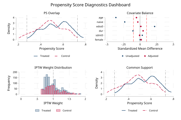
The final FIPTIW analysis weight can be summarized separately with iivwcomponent(final).
psdash console output
. psdash combined, saving("iivw/demo/iivw_psdash_dashboard.png")
Propensity Score Diagnostics Dashboard
Treatment:     tx
PS variable:   _iivw_ps
Covariates:    6
Weights:       _iivw_tw
Estimand:      ATE
Source:        iivw treatment model
Weight component: treatment IPTW (_iivw_tw)

Overlap: Good ( 4.8% outside support)
Balance: Adequate (max |SMD| =  0.055)
Weights: Acceptable (ESS = 94.3% of N)
Support: Good ( 4.8% outside support)
Overall: PASS
. psdash weights, iivwcomponent(final) detail graph ///
    saving("iivw/demo/iivw_psdash_final_weights.png")
IPTW Weight Diagnostics
Weight variable:   _iivw_weight
Weight component:  final FIPTIW (_iivw_weight)
Source:            iivw final analysis weight

Effective Sample Size (ESS)
                                 Overall        Treated        Control
                      ESS         1668.2         1086.4          582.9
               ESS % of N          89.7%          91.6%          86.5%

Weights: Acceptable (ESS = 89.7% of N)
Direct reporting export examples
. iivw_balance, nolog ///
    xlsx("iivw/demo/iivw_reporting_exports.xlsx") sheet("Balance") replace
Balance export: xlsx() sheet Balance
. iivw_exogtest sdmt relapse, ///
    id(id) time(years) ///
    adjust(age female edss0 sdmt0 dur naive) ///
    by(tx) efron nolog ///
    xlsx("iivw/demo/iivw_reporting_exports.xlsx") sheet("Exogeneity") ///
    title("SDMT visit-timing exogeneity diagnostic") ///
    footnote("Outcome-dependent visits; artifact adjustment is a sensitivity range.") ///
    decimals(3)
Exogeneity export: xlsx() sheet Exogeneity decimals 3
. iivw_diagnose years, ///
    unweighted(M_unweighted) weighted(M_fiptiw) adjusted(M_adjusted) ///
    estimand(marginal) exogeneity(endogenous) ///
    excel("iivw/demo/iivw_reporting_exports.xlsx") sheet("Diagnostics") replace
Diagnostic export: excel() sheet Diagnostics
The key diagnostic pattern in the demo mirrors the study logic: weighting moves the marginal/reference time slope only modestly, while the measurement-process adjustment moves it sharply. Because the exogeneity check finds that lagged outcomes predict future visit timing, iivw_diagnose reports a diagnostic range rather than a point artifact share.
Key diagnostic output
. iivw_diagnose years, ///
    unweighted(M_unweighted) weighted(M_fiptiw) adjusted(M_adjusted) ///
    estimand(marginal) exogeneity(endogenous)
IIVW diagnostic decomposition for marginal/reference slope: years

                       Model       Estimate          SE   95% CI
------------------------------------------------------------------------------
                  Unweighted         0.7262      0.0860      0.5577,   0.8947
                    Weighted         0.6566      0.0826      0.4947,   0.8185
    Weighted + artifact adj.        -0.4833      0.2235     -0.9213,  -0.0453
------------------------------------------------------------------------------

Diagnostic movement
Sampling gap:           0.0696
Artifact gap:           1.1398
Total gap:              1.2094

Sampling/artifact shares are not displayed because the measurement
adjustment is marked as potentially endogenous.

Because the measurement process appears outcome-dependent, the adjusted
model may over-correct. Treat the weighted and adjusted estimates as a
diagnostic range, not a point decomposition.
Plausible diagnostic range:   -0.4833 to    0.6566
Categorical-time regtab labels
. iivw_fit sdmt tx age female edss0 dur naive sdmt0 relapse, ///
    model(gee) timespec(categorical) timebasecat(1) ///
    categorical(tx) interaction(tx) replace nolog
Treatment by visit wave
  |  Visit wave: Month 6 (vs. Baseline)    1.03     (0.49, 1.56)    <0.001 |
  | Visit wave: Month 12 (vs. Baseline)    1.56     (1.02, 2.11)    <0.001 |
  | Visit wave: Month 18 (vs. Baseline)    2.12     (1.58, 2.66)    <0.001 |
  |      NTZ-like x Visit wave: Month 6   -0.12    (-0.88, 0.64)      0.75 |
  |     NTZ-like x Visit wave: Month 12   -0.09    (-0.81, 0.63)      0.81 |
  |     NTZ-like x Visit wave: Month 18    0.37    (-0.39, 1.12)      0.34 |

Generated categorical-time terms: _iivw_tcat_1 _iivw_tcat_2 _iivw_tcat_3
Generated treatment-by-wave terms:  _iivw_ix_ntz_like_tcat_1 _iivw_ix_ntz_like_tcat_2 _iivw_ix_ntz_like_tcat_3
  _iivw_ix_ntz_like_tcat_1: NTZ-like x Visit wave: Month 6
  _iivw_ix_ntz_like_tcat_2: NTZ-like x Visit wave: Month 12
  _iivw_ix_ntz_like_tcat_3: NTZ-like x Visit wave: Month 18
The generated model workbook asserts that the Visit waves sheet contains the readable row label NTZ-like x Visit wave: Month 6.
References
- Buzkova P, Lumley T. Longitudinal data analysis for generalized linear models with follow-up dependent on outcome-related variables. Canadian Journal of Statistics. 2007;35(4):485-500. doi:10.1002/cjs.5550350402.
- Lin H, Scharfstein DO, Rosenheck RA. Analysis of longitudinal data with irregular, outcome-dependent follow-up. Journal of the Royal Statistical Society: Series B (Statistical Methodology). 2004;66(3):791-813. doi:10.1111/j.1467-9868.2004.b5543.x.
- Pullenayegum EM. Multiple outputation for the analysis of longitudinal data subject to irregular observation. Statistics in Medicine. 2016;35(11):1800-1818. doi:10.1002/sim.6829.
- Tompkins G, Dubin JA, Wallace M. On flexible inverse probability of treatment and intensity weighting: Informative censoring, variable selection, and weight trimming. Statistical Methods in Medical Research. 2025;34(5):915-937. doi:10.1177/09622802241313289.
Changelog
v1.5.1 (2026-06-11)
- Enforced
decimals()/digits()bounds iniivw_balanceandiivw_diagnosebefore export dispatch - Fixed
iivw_diagnoseworkbook exports so the diagnostics header honors the requestedlevel() - Protected existing workbook sheets from accidental overwrite unless
replaceis specified - Fixed unlabeled negative categorical levels in
iivw_fitso generated dummy names are valid Stata names - Made
entry()validation match the documentednobaseeventbehavior iniivw_weight - Hardened captured display paths so SMCL headings and error-help text do not produce spurious
r(199)returns - Added regression QA for balance thresholds, export footnotes, diagnostics export confidence-level headers, categorical-time
e()metadata, workbook sheet protection, negative categorical levels,nobaseevententry handling, and deterministic diagnostic known answers
v1.5.0 (2026-05-29)
- Persisted the treatment propensity score as
_iivw_psfor IPTW/FIPTIW runs - Added the shared iivw treatment-PS metadata contract consumed by
psdash - Added treatment-component returns from
iivw_weightand_iivw_get_settings - Documented the
psdash combinedhandoff for treatment-propensity diagnostics
v1.4.0 (2026-05-29)
- Added styled
.xlsxsheet export toiivw_exogtest, including variable-label predictor rows, per-group hazard-ratio blocks, joint-test rows, andr(xlsx),r(sheet), andr(decimals)returns - Restyled the direct
iivw_balanceandiivw_diagnoseworkbook sheets to match the tabtools/regtab export layout, including grouped headers and readable row labels - Updated exogeneity QA to verify local package loading, workbook creation, by-group export rows, soft export failure, and
decimals()bounds
v1.3.1 (2026-05-28)
iivw_fitnow errors instead of silently ignoringcollectwhen it is combined withmodel(mixed)orbootstrap(); thecollect:prefix is only applied to non-bootstrapmodel(gee)fits. Added a Stata 17+ guard forcollect- Documented the valid
iivw_diagnose, level()range (greater than 10 and less than 99.99) - Removed unused internal locals in
iivw_diagnose
v1.3.0 (2026-05-27)
- Added
iivw_weight, nobaseevent: treats each subject's first visit as study entry (risk onset) rather than a modeled visit-intensity event. The Andersen-Gill model then fits only follow-up visits, removing the circularity of the baseline visit predicting its own occurrence, and lets single-visit subjects pass through (they contribute a baseline row with weight 1 instead of triggering the "requires at least 2 visits" error). Default behavior is unchanged - Improved the 2-visit error message to point users to
nobaseevent - Stored
r(nobaseevent)and_dta[_iivw_baseevent]to record the mode - Added styled direct
.xlsxsheet reporting exports toiivw_balanceandiivw_diagnose
v1.2.3 (2026-05-26)
- Fixed
iivw_fit, bootstrap()so the bootstrap results table honorslevel(); previously the bootstrapped output always reported 95% intervals while the iivw summary table used the requested confidence level
v1.2.2 (2026-05-26)
- Added
iivw_fit, timespec(categorical)for visit-wave or period indicators, withtimebasecat()to choose the reference time category - Added stable generated categorical-time names and table-ready variable labels for time dummies and time interactions, including categorical predictor x categorical time terms for
collect/regtab - Stored categorical-time metadata in
e()and dataset characteristics, and added QA for generated labels, interactions, andregtabexport
v1.2.1 (2026-05-25)
- Refreshed the diagnostic documentation and demo around the current
iivw_balance,iivw_exogtest, andiivw_diagnoseworkflow
v1.2.0 (2026-05-24)
- Added
iivw_balancefor weight-leverage and visit-model balance diagnostics - Stored expanded visit-model covariates in
iivw_weightmetadata for downstream diagnostics - Added balance QA and updated package command inventory, help, README, and install manifest
v1.1.0 (2026-05-24)
- Added
iivw_fit, unweightedfor fitting the baseline outcome model through the same surface as weighted models - Added
iivw_exogtestto test whether lagged outcomes or disease activity predict future visit/test timing - Added
iivw_diagnoseto compute marginal/reference-slope sampling and measurement-artifact movement across stored models - Added Scenario E QA for nonseparable headroom-dependent measurement artifact
- Updated package overview, help, README, and install manifest for the diagnostic workflow
v1.0.6 (2026-05-18)
- Rejected the panel time variable in
iivw_fitindepvarswhentimespec()also adds it (prevents silent collinear duplication) - Deferred
iivw_weightandiivw_fitmetadata wipes past input validation so validation-stage failures preserve prior weights/fit state - Formatted effects table now shows an
(omitted)row for predictors dropped by the estimator instead of silently skipping them - Added an Intercept row to the formatted effects table
- Fixed
iivw_weight.sthlpabbreviation documentation fortreat_cov()(minimum abbreviation istreat) - Softened convergence-warning advisory lines from
as errortoas text; standardizedexit 198→error 198and removed a dead post-filter line - Added v1.0.6 regression QA covering all of the above
v1.0.5 (2026-05-09)
- Rejected invalid long
generate()prefixes before creating partial outputs - Rejected missing
treat()values for IPTW/FIPTIW and negativebootstrap()counts - Added exact known-answer validation and stricter R fixture coefficient checks
v1.0.4 (2026-05-06)
- Added hard validation that
id()andtime()are nonmissing beforeiivw_weightreachesstset - Enforced
entry()as nonmissing, constant within subject, and strictly earlier than each subject's first visit - Added adversarial QA lanes for weighting, outcome fitting, release/install/docs, validation guards, and external R cross-validation
- Integrated quick/full QA runner modes with full-mode R reference regeneration
v1.0.3 (2026-04-30)
- Allowed IPTW-only weighting for one-row-per-subject datasets
- Required explicit
treat_cov()for IPTW/FIPTIW treatment models - Allowed
iivw_fittime-only and intercept-only weighted outcome models - Expanded the formatted effects summary to include time and interaction terms
- Made cross-validation path resolution robust to running from the package or repository root
v1.0.2 (2026-04-26)
- Added
efronoption toiivw_weightfor Efron tie-handling in the Cox model (matches R's coxph default; Breslow remains the Stata default) - Added
collectoption to non-bootstrap GEE fits iniivw_fitfor Stata's collect framework integration - Improved
stabcov()documentation with guidance on numerator model specification in FIPTIW settings - Added Remarks in
iivw_fit.sthlpfor choosing between GEE and mixed models, and for timespec selection - Expanded
entry()documentation for late-entry/left-truncation designs - Fixed
iivw.sthlpExample 1 to match README (was showing wrong predictors) - Improved error message for time-varying treatment (suggests MSMs as alternative)
Author
Timothy P Copeland, Karolinska Institutet