msm

Version 1.0.4 | 2026-05-29

msm is a Stata suite for inverse-probability-weighted marginal structural models in person-period data. It is designed for longitudinal settings with time-varying treatments and confounders, where standard regression adjustment can be biased by treatment-confounder feedback.

The package covers the full workflow for conventional static-regime MSM analyses: study protocol specification, variable mapping, validation, stabilized weighting, diagnostics, outcome modeling, counterfactual prediction, plotting, reporting, Excel export, and sensitivity analysis.

When to use this package

Use msm when your data have all of these features:

• Longitudinal panel structure — repeated observations per individual over time.
• Time-varying treatment — treatment status can change between periods.
• Time-varying confounders affected by past treatment — the classic "treatment-confounder feedback" problem. A confounder like biomarker level may be affected by prior treatment and also predict future treatment. Standard regression adjustment cannot handle this without bias; IPTW solves it by reweighting.
• Binary treatment and outcome indicators (0/1). Linear and Cox models are also supported for estimation, but the full prediction workflow requires a binary outcome with a pooled logistic model.

If your treatment is assigned at a single point in time (not time-varying), consider Stata's built-in teffects ipw instead.

Requirements

• Stata 16 or later

Installation

After SSC acceptance, install the released package with:

ssc install msm

Until then, install the current Stata-Tools release directly:

capture ado uninstall msm
net install msm, from("https://raw.githubusercontent.com/tpcopeland/Stata-Tools/main/msm") replace

The release ships msm_example.dta as ancillary example data. To copy it into your current working directory, run:

net get msm, from("https://raw.githubusercontent.com/tpcopeland/Stata-Tools/main/msm") replace

Quick Start

This is the shortest complete prediction-ready workflow using the bundled example dataset. It estimates stabilized treatment weights, fits a pooled logistic MSM, and predicts cumulative incidence under always-treated and never-treated strategies.

capture confirm file msm_example.dta
if _rc net get msm, from("https://raw.githubusercontent.com/tpcopeland/Stata-Tools/main/msm") replace
use msm_example.dta, clear

msm_prepare, id(id) period(period) treatment(treatment) ///
    outcome(outcome) covariates(biomarker comorbidity) ///
    baseline_covariates(age sex)

msm_validate

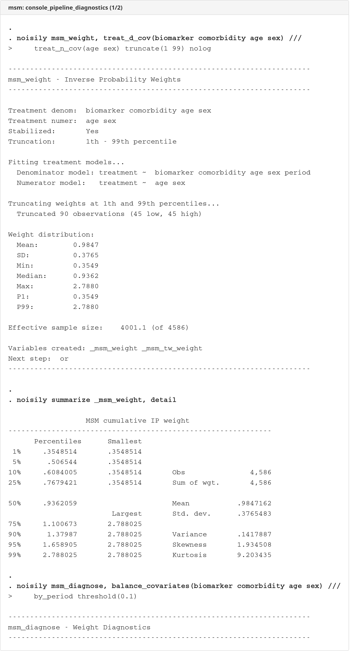
msm_weight, treat_d_cov(biomarker comorbidity age sex) ///
    treat_n_cov(age sex) truncate(1 99) nolog

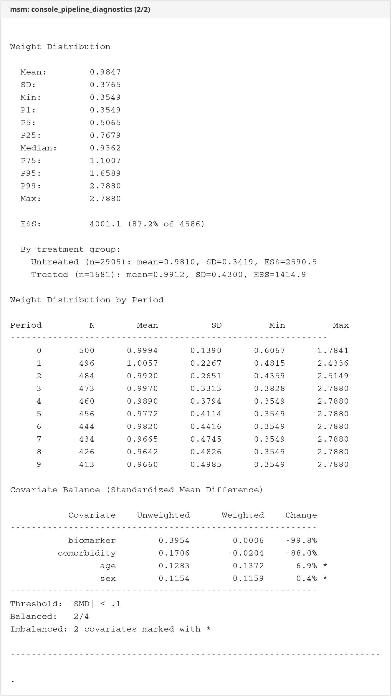
msm_diagnose, balance_covariates(biomarker comorbidity age sex) ///
    by_period

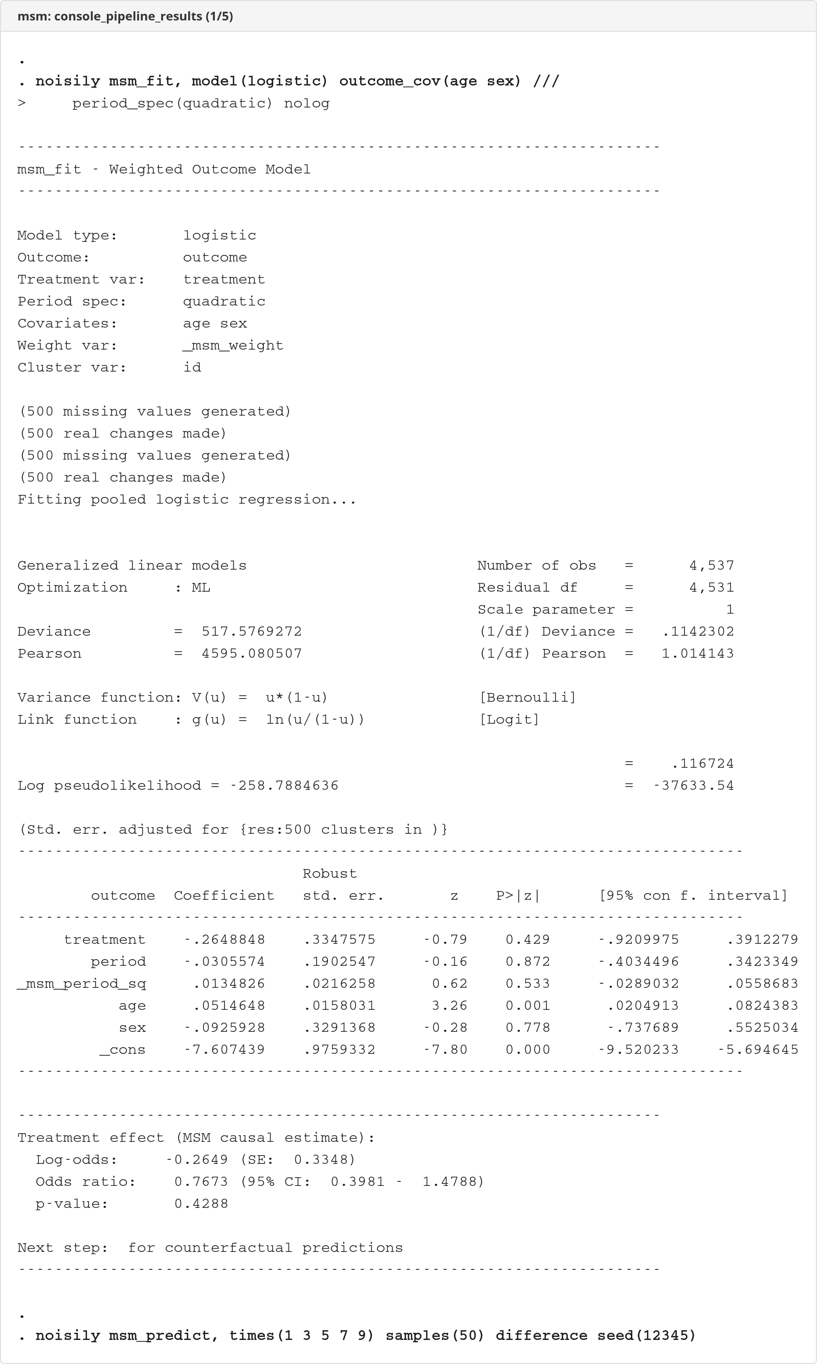
msm_fit, model(logistic) outcome_cov(age sex) nolog

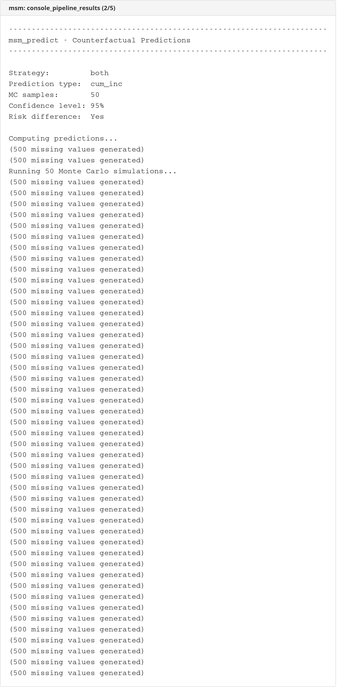
msm_predict, times(1 3 5 7 9) difference seed(12345)

msm_report, eform
msm, status

In plain language, this asks: after accounting for measured time-varying confounding, what would the outcome risk look like if everyone followed the always-treated strategy versus the never-treated strategy?

Commands

Setup and validation

Command	Description
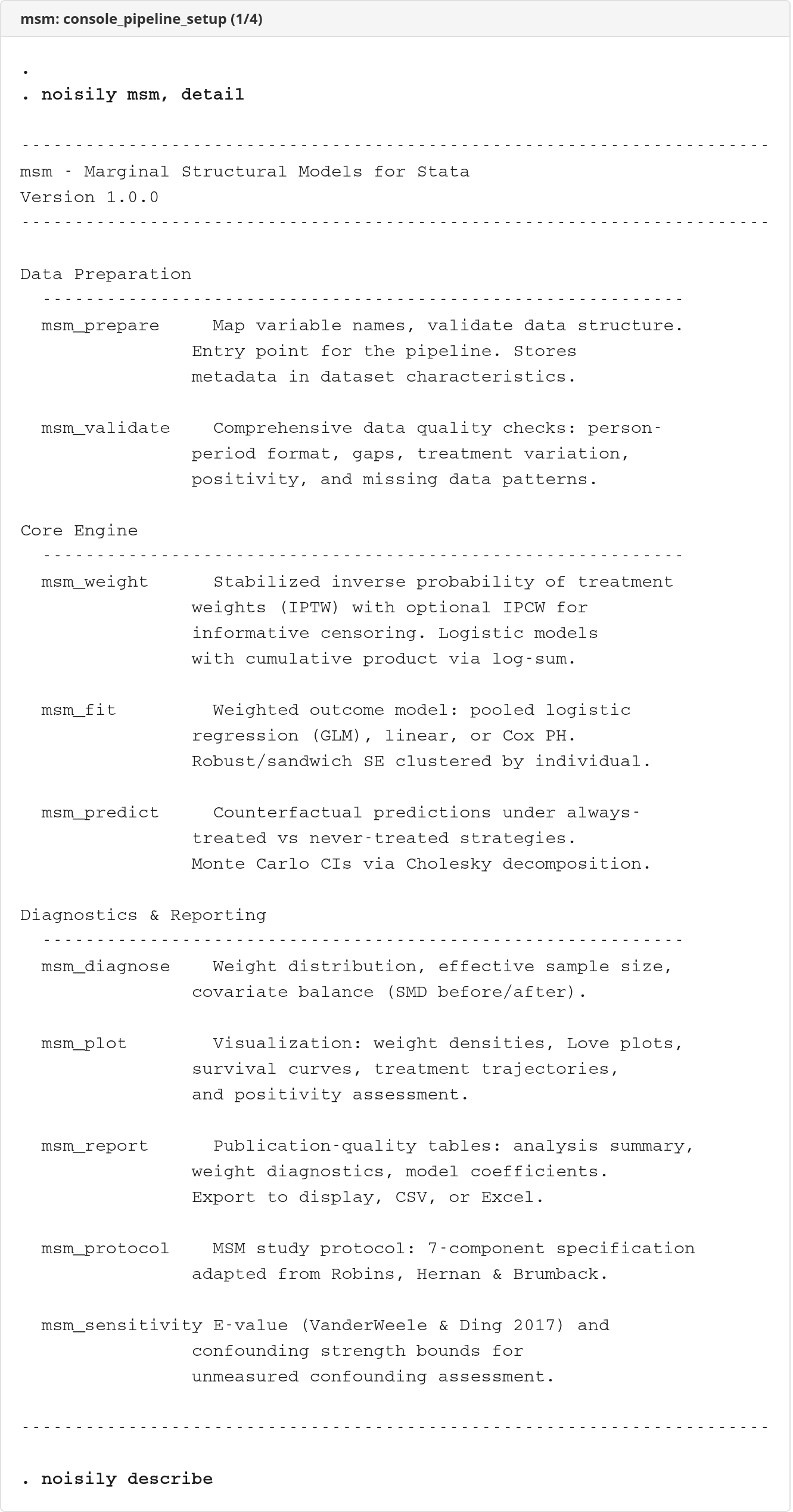
msm	Package overview, workflow guide, and pipeline state check via msm, status
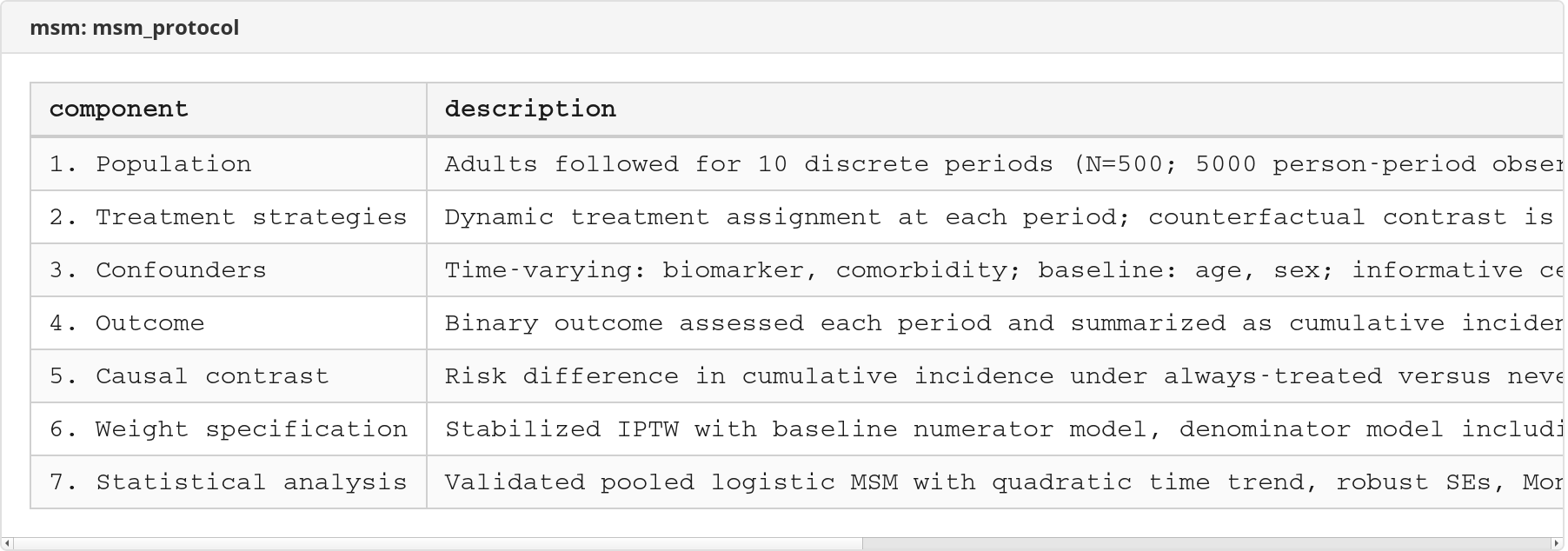
msm_protocol	Record the target trial, causal contrast, weighting plan, and analysis plan (7 components)
msm_prepare	Map identifier, period, treatment, outcome, censoring, and covariate variables
msm_validate	Run 10 data-quality checks for person-period data

Estimation

Command	Description
msm_weight	Estimate stabilized IPTW and optional censoring weights (IPCW)
msm_fit	Fit weighted pooled logistic, linear, or Cox outcome models
msm_predict	Generate counterfactual predictions under always-treated and never-treated strategies

Diagnostics and output

Command	Description
msm_diagnose	Summarize weight distribution and assess covariate balance (SMD before/after)
msm_plot	Draw weight density, Love plot, survival curves, trajectory, and positivity plots
msm_report	Produce a compact publication-style results table (console, CSV, or Excel)
msm_table	Export multi-sheet Excel workbook with all pipeline results
msm_diagtab	Export an accumulated cross-contrast weight-diagnostics summary (one row per contrast) to Excel
msm_sensitivity	Compute E-values and confounding-bound sensitivity summaries

How It Works

msm is organized as a pipeline. Each step stores its results in the dataset as characteristics, matrices, or variables, and downstream commands read those stored artifacts automatically. This means you only specify your variable mapping once (in msm_prepare) and do not need to repeat it at every step.

The pipeline at a glance

msm_protocol  →  msm_prepare  →  msm_validate  →  msm_weight
     ↓                                                  ↓
 (document)                                        msm_diagnose
                                                        ↓
                                                    msm_fit
                                                        ↓
                                                   msm_predict
                                                        ↓
                              msm_plot / msm_report / msm_table / msm_sensitivity

Run msm, status at any point to see the current pipeline stage, what variables are mapped, what artifacts are saved, and what the recommended next step is.

What Should I Run Next?

Situation	Command	Why
You have not mapped the data yet	msm_prepare	Stores which variables are ID, time, treatment, outcome, censoring, and covariates
You want to know whether the data are usable	msm_validate	Checks panel structure, binary variables, missingness, positivity, and outcome timing
You need the pseudo-population	msm_weight	Creates _msm_weight, the stabilized inverse-probability weight used downstream
You are worried about extreme weights or imbalance	msm_diagnose and msm_plot	Summarizes weights and checks whether weighting improved covariate balance
You need the causal effect estimate	msm_fit	Fits the weighted outcome model and stores the treatment effect
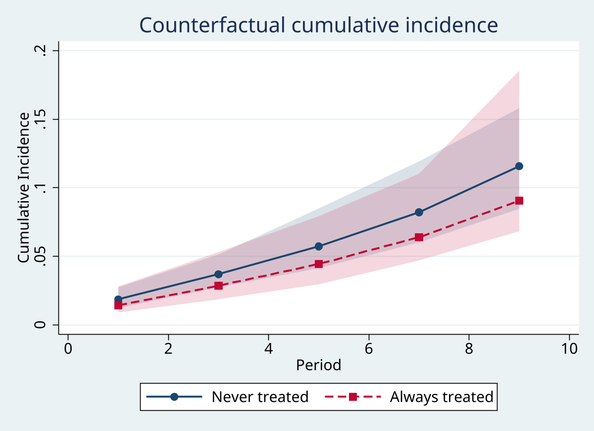
You want absolute risks under treatment strategies	msm_predict	Converts a fitted logistic MSM into standardized counterfactual predictions
You need a paper/report table	msm_report or msm_table	Produces a compact summary or a multi-sheet Excel workbook
You are reopening a saved analysis	msm, status	Shows what has already been run and which artifacts are available

What each step does

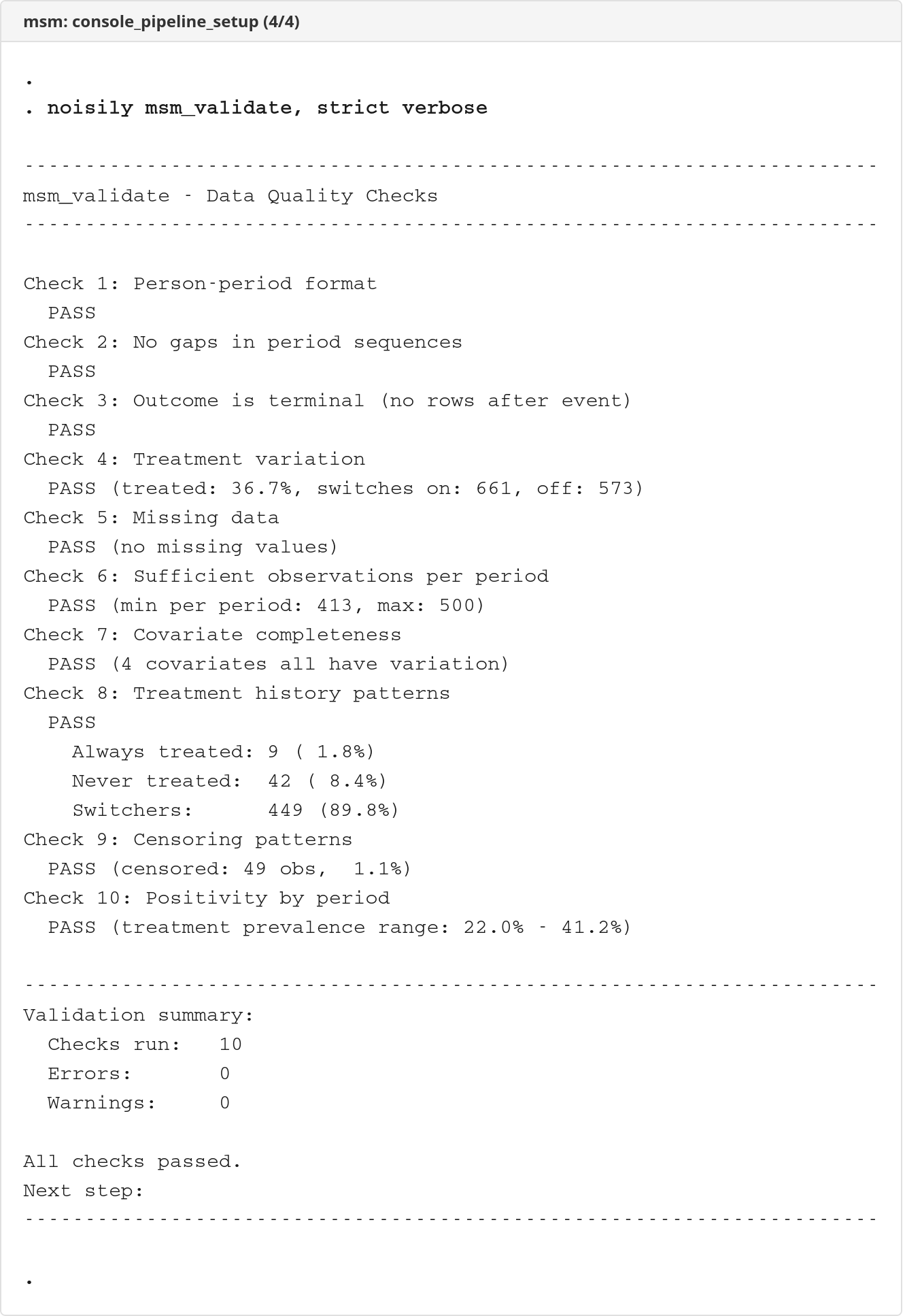
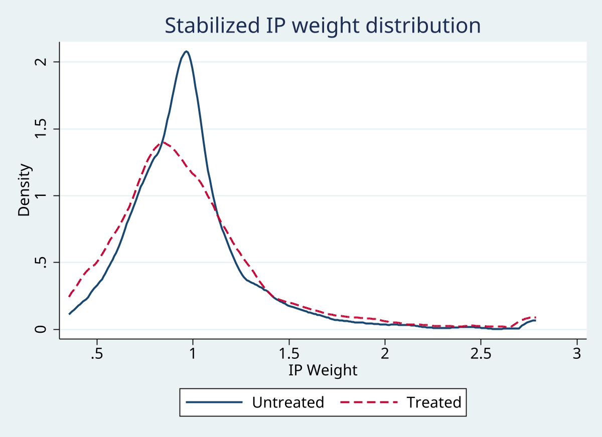
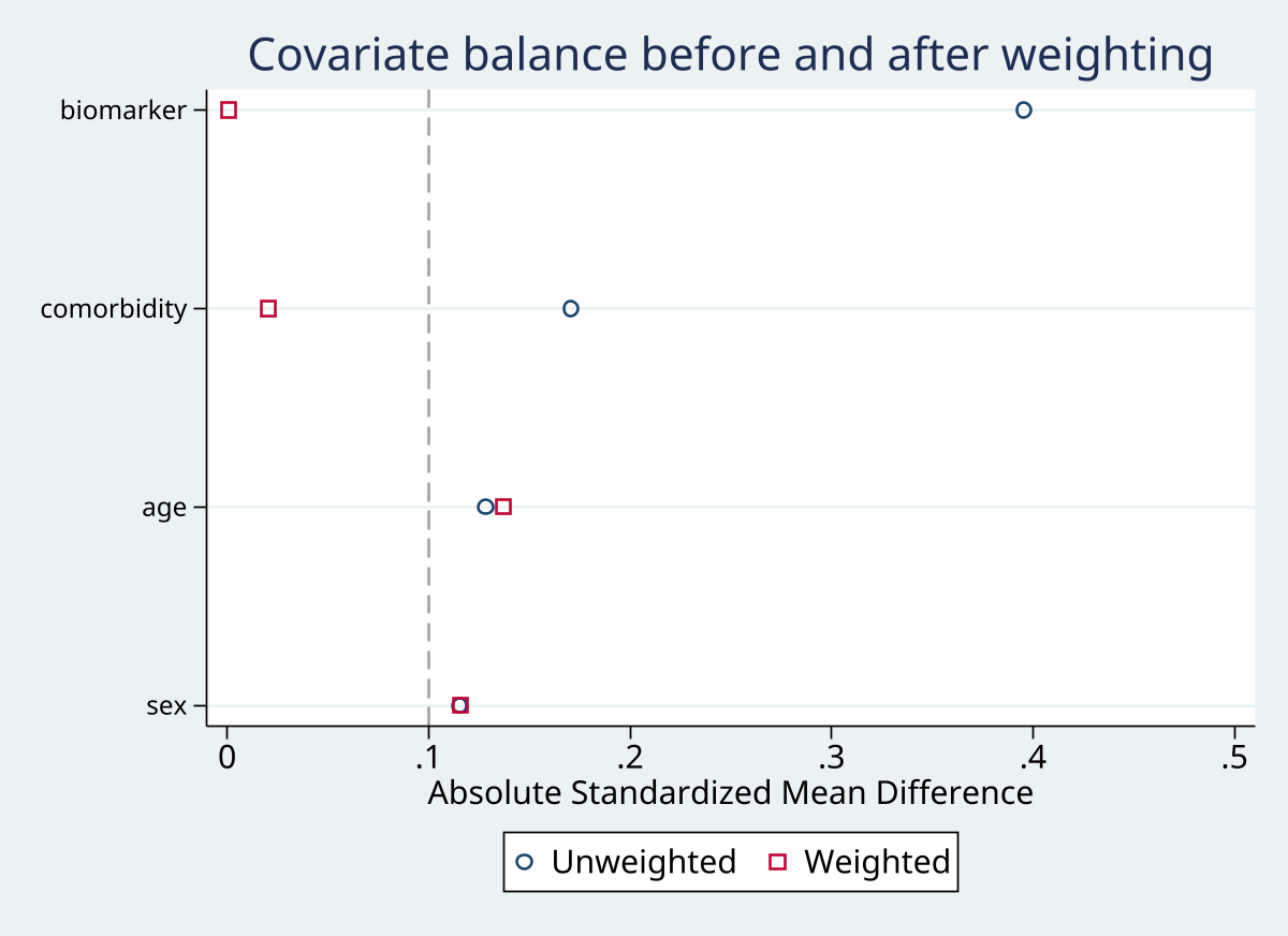
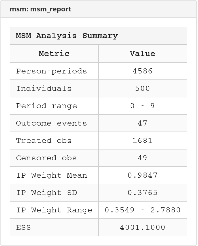
1. msm_protocol — documents the causal question and analysis plan using 7 components adapted from the target trial emulation framework of Hernan et al. (2020). This is purely for documentation; it does not affect computation.

2. msm_prepare — maps your dataset's variable names to roles (ID, period, treatment, outcome, censoring, covariates) and stores the mapping in dataset characteristics. Validates the data structure (person-period format, binary variables, constant baseline covariates). This is the entry point for the analysis.

3. msm_validate — runs 10 data quality checks: person-period format, period gaps, terminal outcomes, treatment variation, missing data, sufficient period sizes, covariate completeness, treatment history patterns, censoring patterns, and positivity by period. Use strict to treat all warnings as hard errors.

4. msm_weight — fits logistic models for the probability of treatment at each period, then combines the period-specific ratios into cumulative stabilized IP weights. Optionally adds censoring weights (IPCW). Truncation at specified percentiles is available to limit the influence of extreme weights.

5. msm_diagnose — reports the weight distribution (mean, SD, percentiles, effective sample size) and computes standardized mean differences (SMD) for each covariate before and after weighting. A good analysis should see SMDs below 0.1 after weighting.

6. msm_fit — fits the weighted outcome model. The treatment coefficient from this model is the MSM causal estimate. Standard errors are robust/sandwich, clustered at the individual level by default, with vce(robust) and vce(cluster varname) available for explicit control.

7. msm_predict — generates standardized counterfactual predictions: "What would the outcome be if everyone were always treated? Never treated?" Uses Monte Carlo simulation from the coefficient distribution for confidence intervals. Risk differences between strategies are available.

8. msm_plot, msm_report, msm_table, msm_sensitivity — visualization, reporting, and sensitivity analysis. msm_table produces a multi-sheet Excel workbook; msm_report produces a single compact summary; msm_sensitivity computes E-values for unmeasured confounding.

Choosing an Outcome Model

msm_fit model	When to use it	Follow-on implications
model(logistic)	Binary outcomes when you also want standardized counterfactual predictions	Required for msm_predict; use msm, status to confirm prediction is available
model(linear)	Binary outcomes on the identity scale when a weighted risk difference is the target	msm_predict is not available; use msm, status to check the current stage before reporting/export
model(cox)	Time-to-event analyses where a weighted hazard ratio is the main estimand	msm_predict is not available; use msm_report, msm_table, msm_sensitivity, and msm, status for pipeline state

msm_fit supports vce(robust) and vce(cluster varname) for weighted linear, pooled logistic, and Cox models. For Cox models, strata(varlist) fits separate baseline hazards by stratum while retaining the treatment effect and requested robust or clustered standard errors.

Data Requirements

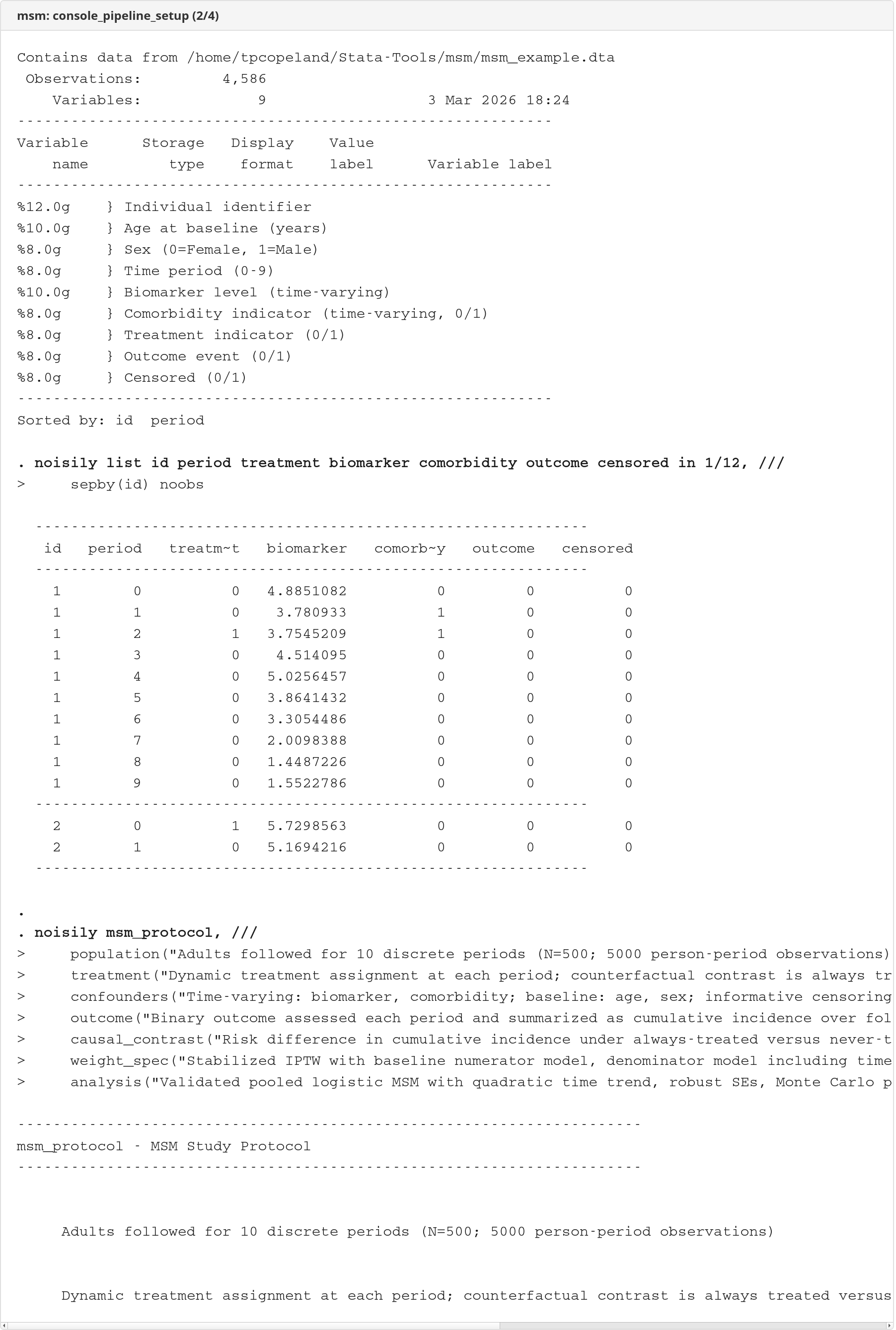
• Data must be in person-period format, with one row per individual-period.
• id() and period() must uniquely identify observations.
• period() must be integer-valued.
• All individuals must share a common baseline period before weighting.
• treatment() and outcome() must be binary 0/1 variables.
• censor() is optional but must also be binary 0/1 when used.
• Variables in baseline_covariates() must be time-fixed (constant within person).
• msm_weight currently rejects delayed entry.
• msm_predict requires a prior msm_fit, model(logistic) run.

Interpreting Key Diagnostics

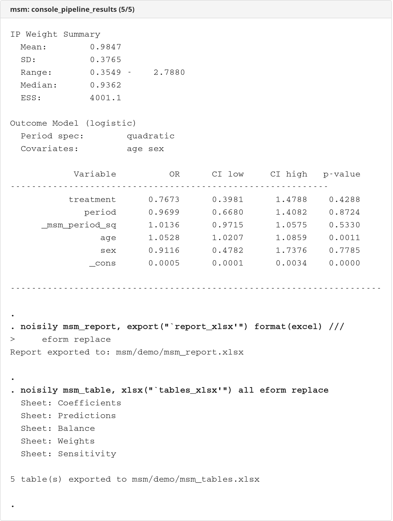
Weight mean

Stabilized IP weights should have a mean close to 1.0. If the mean deviates substantially (e.g., 0.7 or 1.4), the treatment or numerator model may be misspecified. Check your covariate specification.

Effective sample size (ESS)

ESS = (sum of weights)² / (sum of squared weights). It measures how much statistical information the weighted sample retains compared to the original sample. If ESS drops below 50% of N, consider simplifying the weight model or applying stronger truncation.

Standardized mean differences (SMD)

An absolute SMD below 0.1 after weighting is the standard threshold for acceptable covariate balance. SMDs above 0.1 suggest residual confounding for that covariate. If weighting makes balance worse for a variable, investigate the weight model specification.

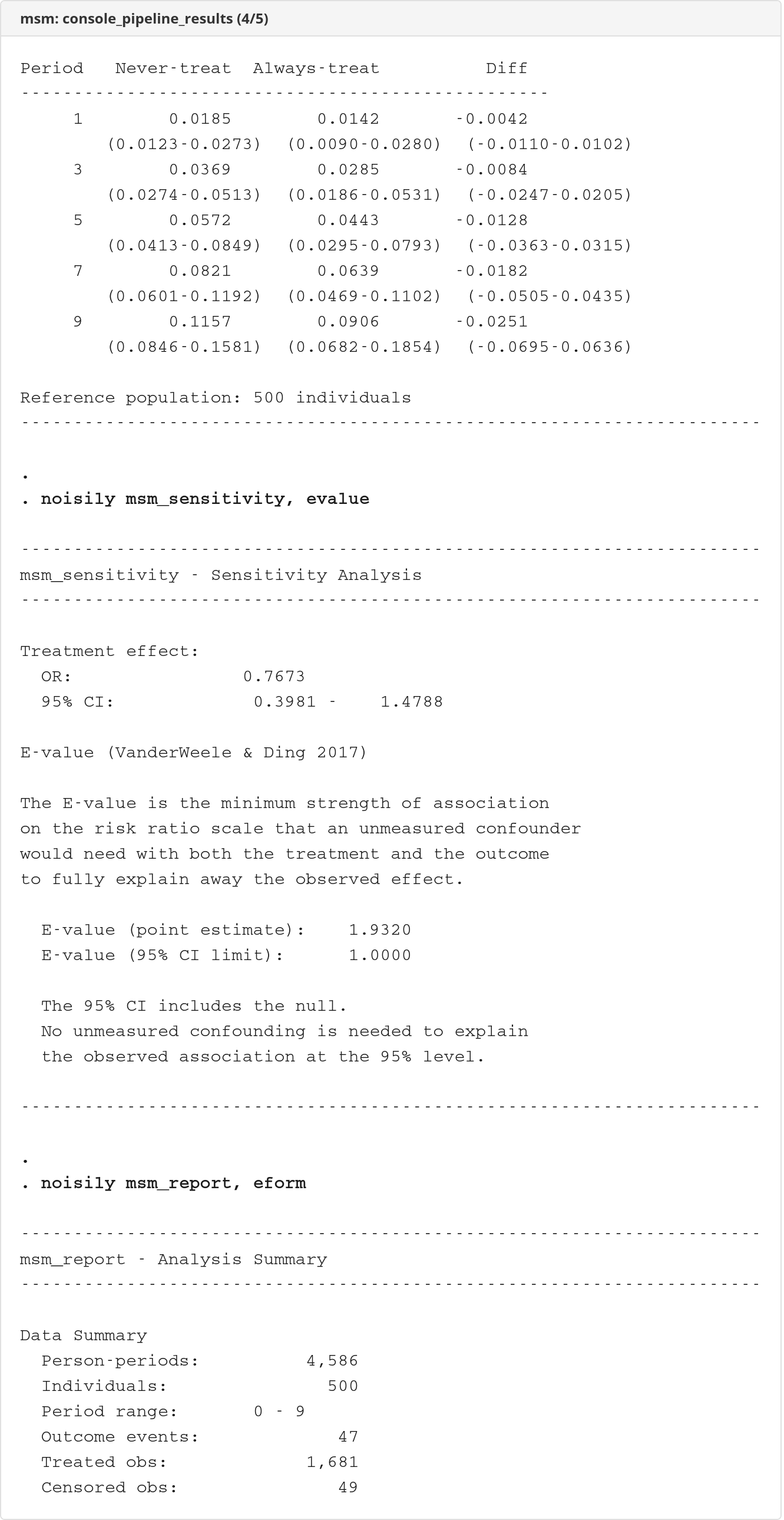
E-value

The E-value is the minimum strength of association (risk ratio scale) that an unmeasured confounder would need with both treatment and outcome to fully explain away the observed effect. An E-value of 1 means the confidence interval already includes the null. E-values above 2-3 indicate the result is moderately to strongly robust to unmeasured confounding.

Current Scope and Limits

• msm targets static binary treatment strategies. Prediction is implemented for always-treated, never-treated, or both; dynamic and stochastic regimes are not supported.
• msm_predict requires a prior msm_fit, model(logistic) run. Linear and Cox fits can be estimated, diagnosed, and reported, but they do not feed into msm_predict.
• outcome_cov() is limited to covariates that are time-fixed within individual; time-varying confounders belong in the weight model.
• msm_weight assumes a shared baseline period. Late entry/left truncation is not supported.
• By default, msm_predict only allows times() within the observed follow-up range. Use extrapolate only when you deliberately want out-of-range predictions.

Demo

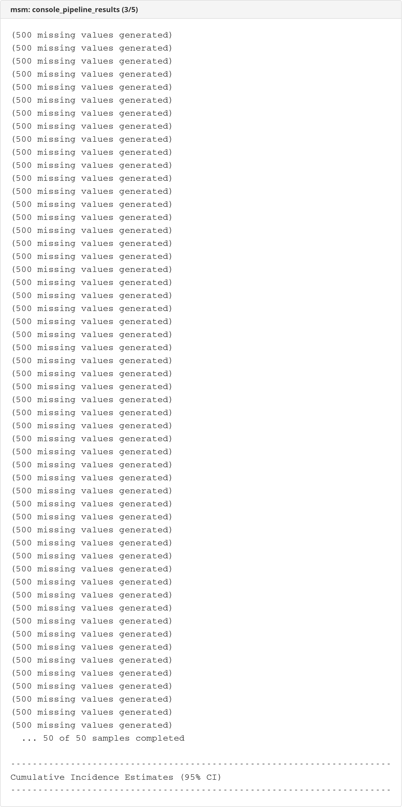
The demo runs the full pipeline on the bundled msm_example.dta dataset. Console output is rendered as self-contained HTML documents using logdoc.

Console output

Setup, protocol, and validation (click to expand)

View HTML | Source .do file

Weighting and diagnostics (click to expand)

View HTML

Estimation, prediction, and reporting (click to expand)

View HTML

Graphs

Excel exports

Excel workbook screenshots (click to expand)

Worked Examples

1. Full pipeline with the bundled example dataset

This example mirrors the package's intended end-to-end workflow. It stays within the supported scope: static always-treat versus never-treat prediction from a pooled logistic MSM.

capture confirm file msm_example.dta
if _rc net get msm, from("https://raw.githubusercontent.com/tpcopeland/Stata-Tools/main/msm") replace
use msm_example.dta, clear

* Step 0: Document the study protocol
msm_protocol, ///
    population("Adults aged 18-65 with condition X") ///
    treatment("Always treat vs. never treat") ///
    confounders("Biomarker (time-varying), comorbidity (time-varying), age, sex") ///
    outcome("Binary clinical endpoint") ///
    causal_contrast("ATE: always treat vs. never treat") ///
    weight_spec("Stabilized IPTW, truncated at 1st/99th percentile") ///
    analysis("Pooled logistic regression, robust SE clustered by ID")

* Step 1: Map variables
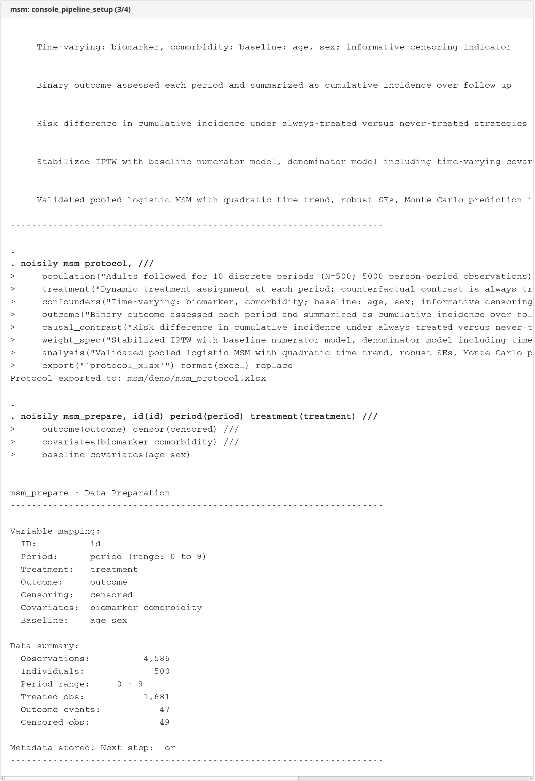
msm_prepare, id(id) period(period) treatment(treatment) ///
    outcome(outcome) covariates(biomarker comorbidity) ///
    baseline_covariates(age sex)

* Step 2: Validate data quality
msm_validate, strict verbose

* Step 3: Calculate stabilized IP weights
msm_weight, treat_d_cov(biomarker comorbidity age sex) ///
    treat_n_cov(age sex) truncate(1 99) nolog

* Step 4: Diagnose weights and balance
msm_diagnose, balance_covariates(biomarker comorbidity age sex) ///
    by_period threshold(0.1)

* Step 5: Fit the weighted outcome model
msm_fit, model(logistic) outcome_cov(age sex) nolog

* Check pipeline state
msm, status

* Step 6: Counterfactual predictions
msm_predict, times(1 3 5 7 9) type(cum_inc) difference ///
    samples(200) seed(12345)

* Step 7: Sensitivity analysis
msm_sensitivity, evalue

* Step 8: Reporting and visualization
msm_plot, type(survival) times(1 3 5 7 9) seed(12345)
msm_report, eform
msm_table, xlsx(msm_results.xlsx) all eform replace

For Excel workbooks, replace in msm_report, msm_table, and msm_protocol replaces only the report/table/protocol sheet(s) being written and preserves unrelated sheets in the same workbook.

2. Minimal estimation-and-prediction workflow

If you want the core causal estimates first, this shorter sequence gets you from prepared data to standardized counterfactual predictions quickly.

capture confirm file msm_example.dta
if _rc net get msm, from("https://raw.githubusercontent.com/tpcopeland/Stata-Tools/main/msm") replace
use msm_example.dta, clear

msm_prepare, id(id) period(period) treatment(treatment) ///
    outcome(outcome) covariates(biomarker comorbidity) ///
    baseline_covariates(age sex)

msm_validate
msm_weight, treat_d_cov(biomarker comorbidity age sex) ///
    treat_n_cov(age sex) nolog
msm_fit, model(logistic) outcome_cov(age sex) nolog
msm, status
msm_predict, times(3 5 7 9) difference seed(12345)

3. Estimation-only workflow (Cox model)

When the target estimand is a weighted hazard ratio and prediction is not needed:

capture confirm file msm_example.dta
if _rc net get msm, from("https://raw.githubusercontent.com/tpcopeland/Stata-Tools/main/msm") replace
use msm_example.dta, clear

msm_prepare, id(id) period(period) treatment(treatment) ///
    outcome(outcome) covariates(biomarker comorbidity) ///
    baseline_covariates(age sex)
msm_weight, treat_d_cov(biomarker comorbidity age sex) ///
    treat_n_cov(age sex) nolog
msm_fit, model(cox) outcome_cov(age sex) nolog
msm_report, eform

Output Notes

• msm_weight creates _msm_weight and returns weight summaries such as r(mean_weight), r(ess), and r(n_truncated).
• msm_diagnose returns a balance matrix in r(balance) when balance_covariates() is specified.
• msm_fit stores the weighted model in e() and records the fitted MSM effect matrix in e(effects).
• msm_predict returns the prediction matrix in r(predictions), risk differences in r(rd_#) when difference is requested, and the seed/state used for the Monte Carlo draws in r(seed) plus r(seed_state).
• msm_table exports formatted Excel workbooks and does not leave Stata returned results; msm_report produces compact summaries to console, CSV, or Excel.

Troubleshooting

Symptom	Likely cause and fix
msm_validate reports period gaps	Check that every person has one row per observed period and that id() plus period() uniquely identifies rows
msm_weight says delayed entry is unsupported	All people must share the same baseline period before weighting
Stabilized weight mean is far from 1	Revisit numerator and denominator model covariates; denominator models should contain measured treatment predictors/confounders
Effective sample size is much smaller than N	Extreme weights are dominating; inspect positivity, simplify the weight model, or consider stronger truncate() values
Balance is still poor after weighting	Add or revise treatment model covariates, check functional form, and inspect by-period balance
msm_predict refuses to run	Prediction requires a prior msm_fit, model(logistic) and prediction times within observed follow-up unless extrapolate is deliberate
msm_table exports fewer sheets than expected	In default/all mode it exports available artifacts; explicitly requested missing sheets produce errors naming the required prior command

References

• Robins JM, Hernan MA, Brumback B. Marginal structural models and causal inference in epidemiology. Epidemiology. 2000;11(5):550-560.
• Hernan MA, Brumback B, Robins JM. Marginal structural models to estimate the causal effect of zidovudine on the survival of HIV-positive men. Epidemiology. 2000;11(5):561-570.
• Cole SR, Hernan MA. Constructing inverse probability weights for marginal structural models. American Journal of Epidemiology. 2008;168(6):656-664.
• VanderWeele TJ, Ding P. Sensitivity analysis in observational research: introducing the E-value. Annals of Internal Medicine. 2017;167(4):268-274.
• Hernan MA, Robins JM. Causal Inference: What If. Boca Raton: Chapman & Hall/CRC, 2020.

Version History

• 1.0.4 (2026-05-29): Added cross-contrast weight diagnostics: msm_diagnose gains accumulate()/contrast()/outcome() to append one summary row per weighted panel to a frame, and the new msm_diagtab command exports that accumulated frame as a single styled Excel sheet
• 1.0.3 (2026-05-06): Added explicit msm_fit vce() control, Cox strata() support, and external R/Python validation of robust and clustered standard errors
• 1.0.2 (2026-05-06): Added adversarial QA for state invalidation, missing treatment/censoring weights, output export restoration, and clarified binary-outcome model scope
• 1.0.1 (2026-04-30): Hardened validation edge cases, time-fixed outcome-covariate enforcement, Cox guidance, and protocol export escaping
• 1.0.0 (2026-04-26): Initial Stata-Tools release of the full MSM workflow suite

Author

Timothy P Copeland, Karolinska Institutet

License

MIT