psdash

Version 1.1.0 | 2026-05-29

Unified diagnostics dashboard for propensity score analyses in Stata. After teffects, cross-sectional tmle, iivw_weight, logit/probit with manually supplied propensity scores from predict, or in fully manual mode, psdash assesses the four standard PS diagnostic domains through one command family: overlap between treatment groups (psdash overlap), covariate balance before and after weighting (psdash balance), weight distribution and effective sample size (psdash weights), and common-support regions (psdash support). psdash combined runs all four and produces a consolidated dashboard. After ltmle, psdash combined switches to a longitudinal table-first diagnostic instead of running pooled cross-sectional panels.

This package exists because PS diagnostics in Stata are scattered across tebalance, user-written helpers, and ad-hoc summarize/tabstat calls, with each step requiring the analyst to re-specify the treatment variable, covariate list, PS variable, and weighting scheme. psdash collapses that friction: when called after teffects, cross-sectional tmle, or iivw_weight, it reads treatment, covariates, propensity scores, and the relevant weighting scheme directly from the estimation or dataset contract. After logit/probit it still pulls treatment and covariates from the estimation context. In fully manual mode, treatment and PS are passed explicitly; covariates() and wvar() are supplied to the subcommands that use those inputs. Auto-generated propensity scores and IPTW weights are created as temporary working variables and are not left behind in the user's dataset.

Balance reporting is deliberately richer than the tebalance summarize default. psdash balance computes raw and weighted standardized mean differences, variance ratios, Kolmogorov-Smirnov statistics, and a Love plot sorted by absolute SMD, with configurable thresholds and Excel export. When a PS is available, it auto-generates IPTW weights for the requested estimand() (default ATE) and displays adjusted columns alongside raw columns, so the user sees immediately how much weighting resolves any imbalance — with nowvar to suppress weighting and wvar() to supply a pre-computed weight variable. Factor and interaction notation (i.var, c.var, ##) is expanded transparently when balance is auto-detected from a fitted logit/probit/teffects model.

The weights subcommand is the complement. psdash weights reports mean, SD, range, percentiles, effective sample size, and extreme-weight counts, with on-the-fly trim(#), truncate(#), and stabilize modifications exposed through generate(name) so the modified weights are kept as a new variable rather than overwriting the original. psdash support assesses common-support regions via manual PS thresholds or the Crump et al. (2009) optimal-trimming rule and can write an in_support indicator for downstream analyses. All subcommands store results in r() and the dashboard output lines use clear status labels plus a "Consider:" action line when follow-up is warranted.

Installation

* Released version from GitHub:
capture ado uninstall psdash
net install psdash, from("https://raw.githubusercontent.com/tpcopeland/Stata-Tools/main/psdash") replace

* Development install from a local checkout:
capture ado uninstall psdash
net install psdash, from("/path/to/psdash") replace

How It Works

psdash is designed to work in seven modes:

• After teffects: treatment, covariates, propensity scores, and the implied weighting scheme are auto-detected from e(). This is the shortest workflow: fit teffects, then run psdash combined or one of the individual subcommands.
• After cross-sectional tmle: treatment, _tmle_ps, covariates, and estimand() are read from the tmle contract state. psdash combined and individual subcommands can be called without retyping those inputs.
• After ltmle: run psdash combined. It reports period-by-period PS overlap and the contract weight distribution using the LTMLE PS and weight variables. Pooled individual subcommands require explicit variables rather than silently treating the longitudinal data as cross-sectional.
• After iivw_weight: treatment, _iivw_ps, treatment-model covariates, and _iivw_tw are read from the iivw dataset contract. Run psdash combined for treatment-propensity diagnostics, then iivw_balance for visit-intensity diagnostics.
• After logit/probit: treatment and covariates are read from the estimation context, but you still supply the PS variable created by predict.
• After mlogit (multi-group): for multi-valued treatments with nonnegative integer levels, treatment and covariates are auto-detected from e(). Run predict ps1 ps2 ps3, pr and pass the GPS variables via psvars(ps1 ps2 ps3).
• Manual mode: provide treatment and PS explicitly, then pass covariates() to balance/combined and wvar() to balance/weights/combined when you want to override auto-detection.

When a PS variable is available, psdash balance auto-generates IPTW weights for the requested estimand() unless you suppress that with nowvar or provide wvar() yourself. Auto-generated propensity scores and weights are temporary working variables and are not left behind in the user's dataset.

Using psdash with iivw

When iivw_weight is run with treat() and treat_cov(), the treatment propensity model can be diagnosed with psdash.

Run psdash combined immediately after iivw_weight to inspect treatment-propensity overlap, common support, treatment-covariate balance, and treatment-weight distribution. Then run iivw_balance for the visit-intensity component. The two diagnostics answer different questions: psdash checks treatment positivity and treatment-model balance; iivw_balance checks whether visit-intensity weights have enough leverage and whether modeled visit covariates are balanced.

iivw_weight, id(id) time(months) ///
    visit_cov(age sex bl_edss bl_sdmt) ///
    lagvars(sdmt relapse) ///
    treat(treated) treat_cov(age sex bl_edss bl_sdmt) ///
    truncate(1 99) efron replace nolog

psdash combined, saving(treatment_ps_dashboard.png)
psdash weights, iivwcomponent(final) graph saving(final_fiptiw_weight.png)
iivw_balance, agrefit nolog
iivw_fit sdmt treated age sex bl_edss, timespec(ns(3)) nolog

What Should I Run?

Most users can start with psdash combined. It runs the four diagnostic panels together and prints an overall status line. If one panel raises a caution, rerun that subcommand by itself to inspect the graph, export a table, or create a modified weight/support variable.

Question	Command	What to look for
Do treated and control observations have comparable propensity scores?	psdash overlap	Large percentages outside common support, very high AUC, PS values near 0 or 1
Are the covariates balanced after adjustment?	psdash balance	Maximum absolute SMD above threshold(); variance ratios outside 0.5 to 2.0; large KS statistics
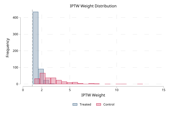
Are a few observations dominating the weighted analysis?	psdash weights	Low ESS, high coefficient of variation, weights above 10 or 20
Which observations are inside the usable support region?	psdash support	Number outside empirical common support and number trimmed by crump or threshold()
Do I need the full dashboard in one step?	psdash combined	Overall PASS/CAUTION plus the panel named in the warning

Reading the Output

psdash uses the same diagnostics that are common in propensity-score reporting, but it labels the output so a non-specialist can follow the next action:

• Overlap/support warnings mean the treatment groups do not share enough comparable observations in part of the propensity-score range. Consider trimming, narrowing the study population, changing the estimand, or revisiting the PS model.
• Balance warnings mean one or more observed covariates still differ after adjustment. Consider model revisions, additional covariates or interactions, a different weighting scheme, or reporting the residual imbalance explicitly.
• Weight warnings mean the estimated effect may be sensitive to a small number of observations. Consider stabilized weights, percentile trimming, truncation, or an estimand with better support.
• A PASS or Adequate label is not a causal proof. It means these observed-diagnostic thresholds were not crossed. Outcome-model assumptions, unmeasured confounding, missing data, and study design still need separate judgment.

Worked Examples

The README keeps one binary and one multi-group workflow. The installed help file (help psdash) remains the authoritative source for complete examples, including teffects, ATT, pre-computed weights, focused option examples, and stored-result details. Full demo console transcripts are linked in the Demo section instead of embedded here.

1. Binary manual workflow with sysuse auto

Estimate the propensity score with logit, save fitted probabilities in ps, then run each diagnostic explicitly. Because this is a manual workflow, balance is told which covariates to assess.

sysuse auto, clear
logit foreign mpg weight length
predict double ps, pr
psdash overlap foreign ps
psdash balance foreign ps, covariates(mpg weight length) loveplot
psdash weights foreign ps
psdash support foreign ps, crump generate(in_support)

After logit or probit, treatment and covariates are still available in e(), so commands that need only the propensity score can also be called as psdash overlap ps, psdash balance ps, loveplot, and psdash weights ps.

2. Multi-group treatment with mlogit

When the treatment has more than two levels, estimate generalized propensity scores and pass the K predicted probabilities through psvars().

clear
set obs 300
set seed 20260506
gen double age = rnormal(60, 10)
gen byte female = runiform() > .5
gen double bmi = rnormal(27, 4)
gen double eta1 = -0.2 + 0.03*(age-60) + 0.25*female - 0.04*(bmi-27)
gen double eta2 = 0.1 - 0.02*(age-60) + 0.02*(bmi-27)
gen double den = 1 + exp(eta1) + exp(eta2)
gen double p0 = 1/den
gen double p1 = exp(eta1)/den
gen double u = runiform()
gen byte arm = cond(u < p0, 0, cond(u < p0 + p1, 1, 2))

mlogit arm age female bmi
predict double ps0 ps1 ps2, pr
psdash overlap arm, psvars(ps0 ps1 ps2)
psdash balance arm, psvars(ps0 ps1 ps2) covariates(age female bmi)
psdash weights arm, psvars(ps0 ps1 ps2) detail
psdash support arm, psvars(ps0 ps1 ps2) threshold(0.1)
psdash balance arm, psvars(ps0 ps1 ps2) covariates(age female bmi) reference(1)

For the automatic teffects workflow, ATT handling, pre-computed weights, and focused option examples, run help psdash after installation.

Subcommands

Subcommand	Purpose
overlap	PS density/histogram by treatment group
balance	SMD balance table + Love plot
weights	Weight distribution, ESS, extreme weights, trim/stabilize
support	Common support assessment, Crump optimal trimming
combined	All diagnostics in a combined dashboard

Key Options

Common and multi-group options

• estimand(ate|att|atc) - target estimand for generated weights. Default is ate; after teffects, the value is read from e(stat) unless supplied explicitly.
• psvars(varlist) - generalized propensity scores for multi-group treatments, meaning K > 2 or K = 2 with non-0/1 treatment levels. Provide one probability variable per nonnegative integer treatment level, ordered by ascending treatment value.
• reference(#) - reference treatment level for pairwise multi-group balance and weight summaries. Default is the smallest observed treatment level.
• saving(filename) - save the graph produced by the relevant subcommand. For combined, this saves the combined dashboard graph.
• scheme(schemename), title(string), name(string), graphoptions(string) - graph styling options where supported by the subcommand.

overlap

• histogram - use overlapping histograms instead of kernel density plots
• bins(#) - histogram bins; default is 30
• bwidth(#) - kernel density bandwidth; Stata's default is used when omitted
• nograph - show the overlap table without drawing a graph

balance

• covariates(varlist) — covariates to assess (auto-detected if omitted)
• wvar(varname) — weight variable (auto-generated from PS if omitted)

Default behavior: When a PS is supplied, balance auto-generates IPTW weights for the requested estimand() (default: ATE) and displays adjusted SMD/VR columns alongside the raw columns. Pass nowvar to see raw balance only, or wvar() to supply a pre-computed weight variable.

• matched - report matched/unweighted balance; mutually exclusive with wvar()
• nowvar, noweights - suppress automatic weight generation and show raw balance only
• loveplot — generate Love plot
• threshold(#) — SMD threshold (default: 0.1)
• ks - display Kolmogorov-Smirnov statistics; KS values are stored either way
• xlsx(filename) — export to Excel
• sheet(string) - Excel sheet name; default is "Balance"
• format(string) - numeric display format for SMD values; default is %6.3f

weights

• wvar(varname) — weight variable (auto-generated from PS if omitted)
• trim(#) — trim at percentile (50–99.9)
• truncate(#) — cap at fixed value
• stabilize — create stabilized weights
• generate(name) — variable for modified weights
• replace - allow generate() to replace an existing variable
• detail — show percentile distribution
• graph — weight distribution histogram
• xlabel(numlist) - custom x-axis labels for the histogram
• iivwcomponent(treatment|final|visit) - choose the stored iivw treatment, final, or visit component for psdash weights

support

• crump — Crump et al. (2009) optimal trimming for binary treatments; use threshold() for multi-group
• threshold(#) — manual PS trimming threshold, strictly between 0 and 0.5
• generate(name) — create an in-support indicator. With crump or threshold(), this marks the trimmed region; otherwise it marks the empirical common-support interval.
• replace - allow generate() to replace an existing variable
• nograph - show the support table without drawing a graph

combined

• nooverlap, nobalance, noweights, nosupport — suppress panels
• threshold(#) — SMD imbalance threshold for the balance panel only

Stored Results

Each subcommand stores results in r(). Technical users can use these values in QA checks, automated reports, or decision rules.

Subcommand	Key scalars/macros	Matrix
overlap	r(N), r(overlap_lower), r(overlap_upper), r(n_outside), r(pct_outside), r(auc), r(treatment), r(psvar), r(source)	none
balance	r(max_smd_raw), r(max_smd_adj), r(max_vr_raw), r(max_vr_adj), r(max_ks_raw), r(n_imbalanced), r(threshold), r(wvar), r(source)	r(balance)
weights	r(mean_wt), r(sd_wt), r(cv), r(ess), r(ess_pct), r(n_extreme), r(p1), r(p99), r(wvar), r(source), r(iivwcomponent), r(generate)	none
support	r(lower_bound), r(upper_bound), r(n_outside), r(pct_outside), r(trim_lower), r(trim_upper), r(n_trimmed), r(crump_alpha), r(source)	none
combined	Inherits subcommand results via return add; also stores r(treatment), r(psvar), r(wvar), r(estimand), r(source), r(iivwcomponent), and for multi-group runs r(K), r(levels), r(reference)	inherited when balance runs
combined after ltmle	Stores LTMLE metadata (r(longitudinal), r(period), r(periods), r(id), r(wvar), r(method), r(contract_version)), weight diagnostics (r(mean_wt), r(ess), r(ess_pct), percentiles), and r(max_pct_outside)	r(overlap_by_period), r(weights_by_period)

For binary treatments, r(balance) has one row per covariate and columns for raw and adjusted means, SMDs, variance ratios, and KS statistics. For multi-group treatments, r(balance) has one five-column block per non-reference group, plus adjusted blocks when weights are applied; column names include the compared treatment levels.

Example:

psdash balance foreign ps, covariates(mpg weight length)
return list
matrix list r(balance)
* Example decision rule for your own analysis:
* assert r(max_smd_adj) < 0.1

Relationship to Existing Packages

psdash balance incorporates the computation from balancetab and psdash weights from iptw_diag. Both use identical methods. The overlap and support subcommands are new.

Demo

Demo output is generated from demo/demo_psdash.do. Run it from the Stata-Tools repo root with stata-mp -b do psdash/demo/demo_psdash.do. The README links to curated console markdown instead of embedding the full transcripts.

Binary treatment (2 groups)

Synthetic data: 800 observations, confounded treatment assignment, propensity scores via logit, IPTW weights, a continuous outcome for the automatic teffects workflow, and generated support/modified-weight variables.

Output	Console markdown	Image
Overlap diagnostics	demo/console_overlap.md
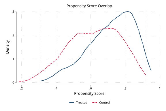Overlap histogram	demo/console_overlap.md
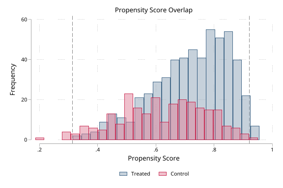Balance and weight diagnostics	demo/console_balance_weights.md
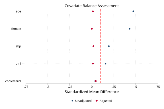Detailed and modified weights	demo/console_weight_options.md
Common support assessment	demo/console_support.md
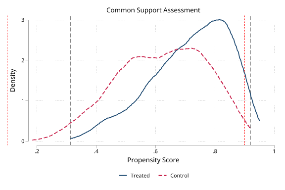Stored results and balance matrix	demo/console_return_values.md
Combined dashboard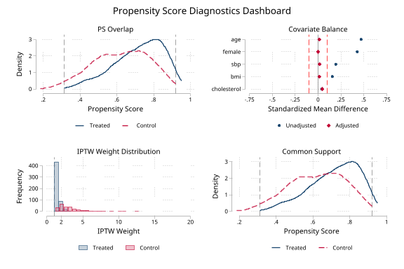
Automatic workflow after teffects	demo/console_teffects_auto.md

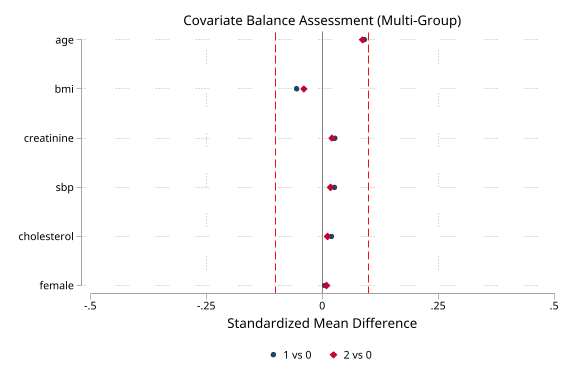
Multi-group treatment (3 arms)

Synthetic data: 1,200 observations, a 3-arm treatment assigned via multinomial logit, generalized propensity scores via mlogit, generalized IPTW weights, threshold-based support indicators, and an alternate reference-arm balance check.

Output	Console markdown	Image
Multi-group overlap	demo/console_mg_overlap.md
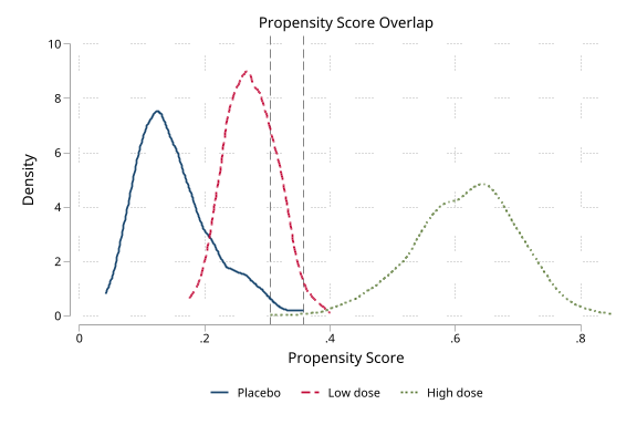Multi-group balance	demo/console_mg_balance.md
Multi-group weight diagnostics	demo/console_mg_weights.md
Multi-group common support	demo/console_mg_support.md
Multi-group reference arm change	demo/console_mg_reference.md
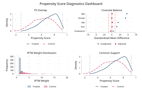
Multi-group combined dashboard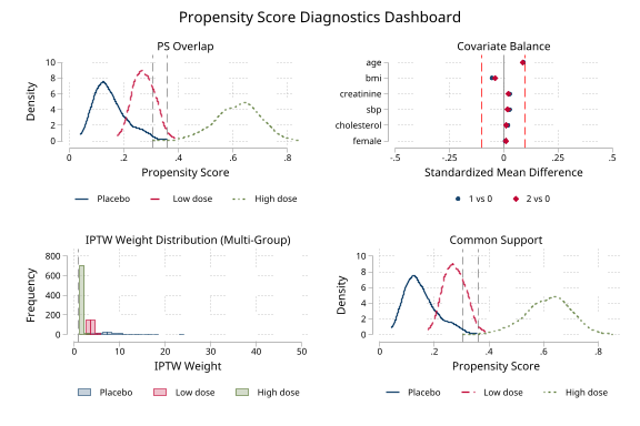

Version History

• v1.1.0 (29 May 2026): Added iivw dataset-contract auto-detection, psdash weights, iivwcomponent(), iivw source labels, and focused iivw contract QA.
• v1.0.2 (17 May 2026): Rejected invalid manual estimand() values, added clean multi-group treatment-level validation, isolated remaining QA installs, and made the demo path handling relocatable with failure-safe cleanup.
• v1.0.1 (06 May 2026): Hardened PS detection and validation, fixed teffects binary PS orientation, K=2 non-0/1 auto-weights, support threshold validation, and binary variance-ratio summaries.
• v1.0.0 (29 Apr 2026): Initial release with five subcommands