raincloud
Reporting & VisualizationRaincloud plots: density, scatter, and box elements
Version 1.0.3 | 2026-08-11
raincloud combines a kernel-density cloud, jittered observations, and a box-and-whisker summary in one graph. It is for Stata users comparing distribution shape, raw values, and robust summaries across one or more groups.
Quick Start
Compare fuel-efficiency distributions for domestic and foreign cars with Stata's built-in data:
sysuse auto, clear
raincloud mpg, over(foreign) seed(2026)
The graph shows the density, observed MPG values, and quartile summary for each origin group. seed(2026) makes the point jitter reproducible for this plot.
Requirements
- Stata 16 or later
- No external packages or software
Installation
Install the released package directly from the public Stata-Tools repository:
capture ado uninstall raincloud
net install raincloud, from("https://raw.githubusercontent.com/tpcopeland/Stata-Tools/main/raincloud") replace
Commands
| Command | Description |
|---|---|
raincloud |
Draw a raincloud plot from one numeric variable |
How It Works
Each plot combines three views of the same distribution: a half-violin kernel density (cloud), jittered raw observations (rain), and a box-and-whisker summary (box).
Without over(), all marked observations are shown as one group. With over(varname), the command creates one raincloud per numeric or string group and uses value labels when available.
The default orientation is horizontal, with the outcome on the x-axis and groups on the y-axis. vertical places the outcome on the y-axis and groups on the x-axis; mirror draws a full mirrored violin with density on both sides of the group center.
The cloud is estimated with Stata's kdensity, the rain layer uses scatter, and the box elements are assembled from group-wise quartiles, medians, means, and whisker endpoints. The command temporarily works on the marked sample and restores the data after drawing the graph.
Worked Examples
1. Single distribution
sysuse auto, clear
raincloud mpg, seed(2026)
With no over() option, the command draws one raincloud and labels the group All.
2. Grouped comparison
sysuse auto, clear
raincloud mpg, over(foreign) seed(2026) title("MPG by car origin")
Use over() when the comparison concerns spread, skewness, overlap, or outliers as well as the center of the distribution.
3. Vertical layout with a mean marker
sysuse auto, clear
raincloud price, over(foreign) vertical mean seed(2026)
mean adds a filled marker at each group mean while the box retains the median and IQR summary.
4. Mirror density without points or boxes
sysuse auto, clear
raincloud mpg, over(foreign) mirror norain nobox seed(2026)
This produces a full mirrored-violin display of the group densities. At least one of the cloud, rain, or box elements must remain enabled.
5. Weights and element styling
sysuse auto, clear
gen int fw = max(1, round(price / 1000))
raincloud mpg [fweight = fw], over(foreign) seed(2026) ///
    cloudopts(lwidth(medium) lpattern(dash)) ///
    pointopts(msymbol(d) msize(tiny)) ///
    boxopts(lwidth(thick)) ///
    title("Weighted fuel efficiency")
fweight and aweight are supported. The three element-specific options pass graph options to the cloud, points, and box whisker line.
Demo
The figures below are generated by demo/demo_raincloud.do from a Stata-Tools repository checkout; the demo script and images are checkout assets rather than part of the net install payload.
| Figure | Focus |
|---|---|
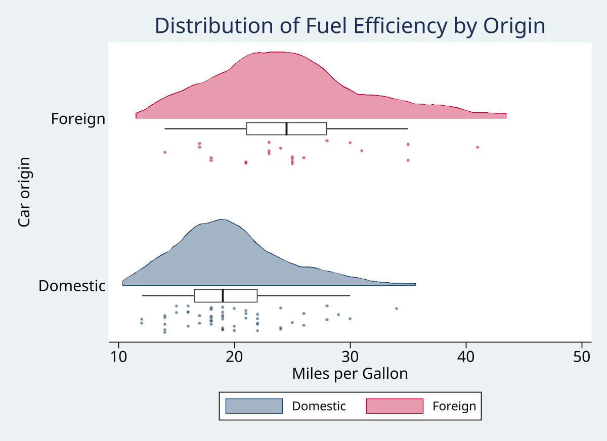 |
Grouped horizontal plot |
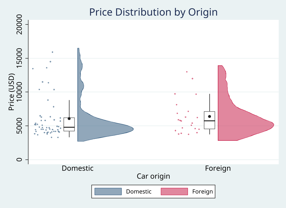 |
vertical and mean |
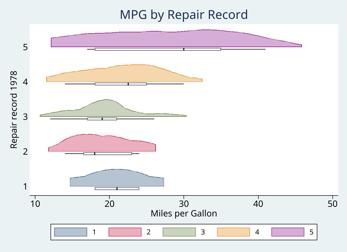 |
norain with five groups |
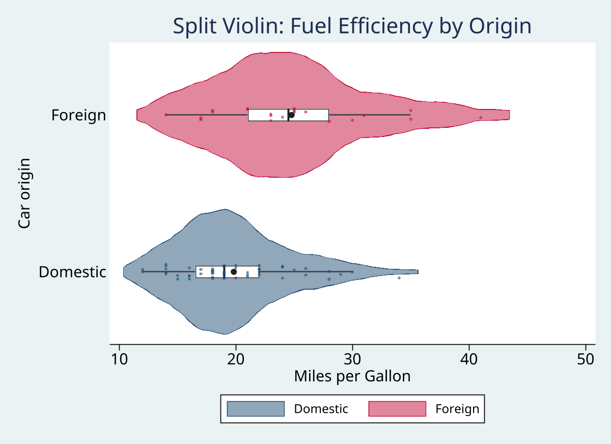 |
mirror and mean |
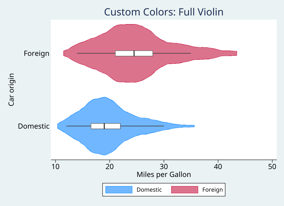 |
colors() and norain |
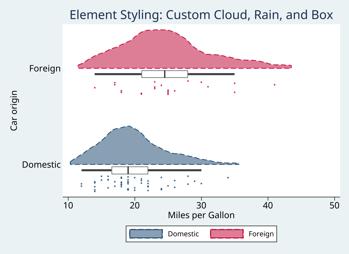 |
cloudopts(), pointopts(), and boxopts() |
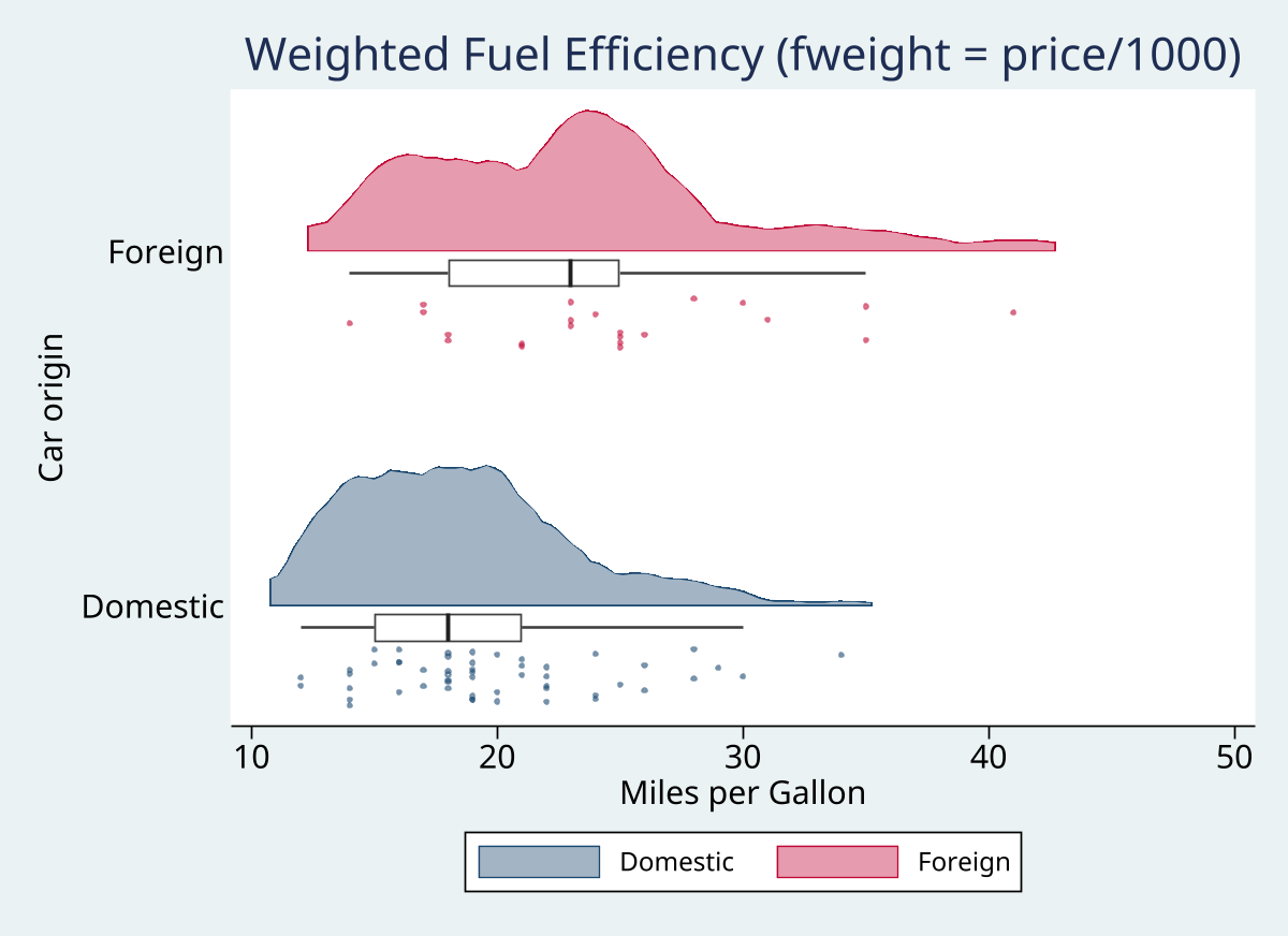 |
fweight support |
From the repository root, run the generator with:
do raincloud/demo/demo_raincloud.do
Command Reference
Syntax
raincloud varname [if] [in] [fweight aweight], ///
    [over(varname) nocloud norain nobox noumbrella ///
     bandwidth(#) kernel(string) n(#) opacity(#) cloudwidth(#) cloudopts(string) ///
     jitter(#) seed(#) pointsize(string) pointopts(string) ///
     boxwidth(#) boxopts(string) nomedian mean ///
     overlap mirror horizontal vertical gap(#) colors(string) ///
     title(string) subtitle(string) note(string) name(string) saving(string) ///
     scheme(string) plotregion(string) graphregion(string) ///
     ytitle(string) xtitle(string) legend(string) *]
The command accepts exactly one numeric varname, optional if/in restrictions, and optional fweight or aweight expressions. The final * accepts additional options documented under Stata's twoway_options.
Key Options
Elements
| Option | Purpose | Default |
|---|---|---|
nocloud |
Suppress the half-violin kernel density | Off |
norain |
Suppress the jittered raw observations | Off |
nobox |
Suppress the box-and-whisker summary | Off |
noumbrella |
Synonym for nobox |
Off |
Cloud
| Option | Purpose | Default |
|---|---|---|
bandwidth(#) |
Use a nonnegative bandwidth for kdensity; 0 uses Stata's optimal selector |
0 |
kernel(string) |
Select any kernel accepted by kdensity |
epanechnikov |
n(#) |
Set the number of density evaluation points; must be at least 10 | 200 |
opacity(#) |
Set cloud fill opacity from 0 (transparent) to 100 (opaque) | 50 |
cloudwidth(#) |
Set the maximum density width in axis units; must be positive | 0.4 |
cloudopts(string) |
Pass options to the cloud's underlying rarea layer |
None |
Rain
| Option | Purpose | Default |
|---|---|---|
jitter(#) |
Set point-jitter intensity from 0 to 1 | 0.4 |
seed(#) |
Set the jitter seed; -1 uses the current state, nonnegative values make the plot reproducible |
-1 |
pointsize(string) |
Set the marker size for the rain layer | vsmall |
pointopts(string) |
Pass options to the rain layer's underlying scatter command |
None |
Box
| Option | Purpose | Default |
|---|---|---|
boxwidth(#) |
Set the IQR box width in axis units; must be positive | 0.08 |
boxopts(string) |
Pass options to the box whisker line | None |
nomedian |
Suppress the median line inside the box | Off |
mean |
Add a filled marker at the group mean | Off |
Layout
| Option | Purpose | Default |
|---|---|---|
over(varname) |
Stratify the plot by a numeric or string grouping variable | None |
horizontal |
Put the outcome on the x-axis and groups on the y-axis | On |
vertical |
Put the outcome on the y-axis and groups on the x-axis | Off |
gap(#) |
Set group spacing at positions 1*gap, 2*gap, and so on; must be positive |
1.0 |
overlap |
Place jittered points over the box instead of offset from it | Off |
mirror |
Draw the cloud on both sides of the group center | Off |
colors(string) |
Supply a space-separated list of Stata color names; colors cycle across groups | navy cranberry forest_green dkorange purple teal maroon olive_teal |
Graph and twoway options
| Option | Purpose | Default |
|---|---|---|
scheme(string) |
Select the graph scheme | Current Stata scheme |
title(string) |
Add a graph title | None |
subtitle(string) |
Add a graph subtitle | None |
note(string) |
Add a graph note | None |
name(string) |
Assign a graph name | None |
saving(string) |
Save the graph to a file | None |
plotregion(string) |
Pass plot-region options to the graph | Default |
graphregion(string) |
Pass graph-region options to the graph | Default |
xtitle(string) |
Set the x-axis title | Outcome label/name when horizontal; group label/name when grouped vertical |
ytitle(string) |
Set the y-axis title | Group label/name when grouped horizontal; outcome label/name when vertical |
legend(string) |
Set legend options; grouped plots otherwise receive an automatic legend | Off for one group; automatic for multiple groups |
* |
Pass any additional twoway_options to the graph command |
As specified |
Stata's normal option-abbreviation rules apply; the full option names above are recommended in scripts. The command rejects simultaneous horizontal and vertical, and it rejects a call that suppresses all three elements.
Stored Results
After a successful call, raincloud displays a short summary of the plotted variable, groups, observations, and active elements and stores the following in r():
| Result | Type | Contents |
|---|---|---|
r(N) |
Scalar | Number of observations in the marked sample after if/in restrictions and missing-value exclusion |
r(n_groups) |
Scalar | Number of groups; 1 when over() is omitted |
r(varname) |
Local macro | Name of the plotted numeric variable |
r(over) |
Local macro | Name of the grouping variable when over() is specified; absent otherwise |
r(group_levels) |
Local macro | Numeric group values used internally, in plot order |
r(group_labels) |
Local macro | Exact group labels, in plot order |
r(stats) |
Matrix | Group-wise summary statistics with columns n, mean, sd, median, q25, q75, iqr, and bandwidth |
Rows of r(stats) correspond to the groups in the plot and use group labels when every label is a valid Stata matrix row name. If any label cannot be represented, including labels longer than 32 characters, all rows receive stable names such as group1 and group2; r(group_labels) preserves the exact label-to-row mapping. bandwidth contains the estimated kdensity bandwidth when a cloud is computed and is missing when density estimation is suppressed or skipped for a group.
With fweight, r(N) counts marked input rows while the n column of r(stats) contains the weighted frequency count. If graph rendering or saving() fails after the analytical calculations, the command returns the graph error code while retaining the analytical results in r() for diagnosis.
For example:
sysuse auto, clear
raincloud mpg, over(foreign) seed(2026)
return list
matrix list r(stats)
Assumptions and Limits
- The plotted variable must be numeric, and only one outcome variable can be supplied.
over()accepts numeric or string variables. Observations missing the outcome or grouping value are excluded from the plot and stored counts.- Groups with one observation or zero variance skip the cloud. A density estimate for a group with fewer than five observations may be unreliable.
- The default palette has eight colors; if fewer colors than groups are supplied, the palette cycles from the beginning.
bandwidth()must be nonnegative,opacity()must be between 0 and 100,jitter()between 0 and 1,n()must be at least 10, andcloudwidth(),boxwidth(), andgap()must be positive.- Omit
seed()to use the current random-number state; the jitter consumes that state. Withseed(#), the command saves and restores the caller's random-number state after drawing;-1is the only negative value allowed. - The command supports
fweightandaweightexpressions and preserves the data andvarabbrevsetting after execution. Withfweight,r(N)counts marked input rows andr(stats)[, "n"]contains weighted frequency counts. - For very large datasets, consider
norainto avoid rendering many points or reducen()to shorten density estimation.
References
- Allen M, Poggiali D, Whitaker K, Marshall TR, Kievit RA. 2019. Raincloud plots: a multi-platform tool for robust data visualization. Wellcome Open Research 4:63. doi:10.12688/wellcomeopenres.15191.1
QA
QA suites are available in qa/.
Version History
- 1.0.3 (2026-08-11): Preserves analytical results after graph-side failures, supports long group labels through stable row names plus exact label metadata, and corrects mirrored-violin terminology
- 1.0.2 (2026-08-05): Rejects missing and negative seeds without changing the caller's RNG state
- 1.0.1 (2026-08-05): Corrected shipped help metadata, documented graph options, and validated bandwidth and seed boundaries
- 1.0.0 (2026-07-10): Initial Stata-Tools release of
raincloud
Author
Timothy P Copeland, Karolinska Institutet
License
MIT