tabtools
Reporting & VisualizationPublication-ready Excel tables (table1_tc, regtab, effecttab, stratetab, tablex)
Version 1.6.4 | 2026-06-10
tabtools is a suite of Stata commands for exporting manuscript-ready tables to Excel and Markdown across descriptive summaries, regression models, treatment effects, survival analysis, diagnostic accuracy workflows, incidence rates, and composite tables. The package is organized around a shared formatting layer, so commands that come from very different analysis pipelines still produce tables that look like they belong in the same workbook or report.
Requirements
- Stata 16 or later for
tabtools,tabtools_tips,table1_tc,stacktab, andsimtab - Stata 17 or later for
desctab,regtab,effecttab,comptab,hrcomptab,survtab,crosstab,corrtab,diagtab,stratetab, andputtab desctab,regtab, andeffecttabrequire Stata'scollectframeworksurvtabrequiresstsetdata, andstratetabexpects savedstrate, output()datasetseplotis optional and is required only when usingcomptab, forestorhrcomptab, forest
Installation
capture ado uninstall tabtools
net install tabtools, from("https://raw.githubusercontent.com/tpcopeland/Stata-Tools/main/tabtools") replace
After installation, start with help tabtools for the suite overview and tabtools_tips for the merged quick reference and worked recipes. The older help tabtools_cheatsheet and help tabtools_cookbook topics still work as compatibility aliases.
Markdown Export
Every table-producing command accepts markdown(filename) to write the rendered table as GitHub-Flavored Markdown. Use mdappend to append several tables into one report file. Markdown can be requested alone where a workbook is not structurally required, or in the same call as xlsx()/excel(), csv(), and frame().
table1_tc age bmi sex, by(treated) markdown("table1.md")
regtab, xlsx("models.xlsx") markdown("models.md")
crosstab sex treated, markdown("tables.md")
corrtab age bmi sbp, markdown("tables.md") mdappend
Commands
Direct table builders
| Command | Description | Stata |
|---|---|---|
table1_tc |
Table 1 generator with automatic tests, SMDs, weighting support, and Excel export | 16+ |
desctab |
Format active table collections with per-statistic formats and composite cells |
17+ |
crosstab |
Cross-tabulation with association measures such as OR, RR, and risk difference | 17+ |
corrtab |
Correlation matrix with significance stars, p-values, and lower, upper, or full layouts | 17+ |
survtab |
Kaplan-Meier survival summary table with medians, RMST, and number at risk | 17+ |
diagtab |
Diagnostic-accuracy table with sensitivity, specificity, predictive values, likelihood ratios, and optional AUC | 17+ |
Post-estimation formatters
| Command | Description | Stata |
|---|---|---|
regtab |
Format the current collect from regression models into a polished table with Excel export and automatic console display, including multi-equation models such as mlogit, zip, zinb, and churdle |
17+ |
effecttab |
Format teffects or margins results from the current collect into an effects table |
17+ |
File and frame workflow builders
| Command | Description | Stata |
|---|---|---|
stratetab |
Format saved strate, output() files into incidence-rate tables |
17+ |
comptab |
Combine selected rows from one or more regtab or effecttab frames into one composite sheet |
17+ |
hrcomptab |
Build a final Table 2-style sheet by combining a stratetab frame with selected regtab rows |
17+ |
Styled export and assembly
| Command | Description | Stata |
|---|---|---|
puttab |
Style a table already in memory — the current dataset, a named frame, or a Stata matrix (e(b), r(table), collapse/tabulate output) — as one house-styled Excel sheet. Feeds stacktab |
17+ |
stacktab |
Assemble multi-sheet composite Excel tables from source blocks (vstack/hstack, column merges, titles, notes). | 16+ |
puttab vs comptab vs stacktab
These three commands all produce a single combined or styled sheet, but they differ by what they read:
| Command | Reads | Level | Use when |
|---|---|---|---|
puttab |
one table already in memory — dataset, frame(), or matrix() (e(b), r(table), collapse/tabulate) |
raw input → one styled sheet | you have a raw table and no specialized command fits; you just want it styled |
comptab |
tabtools regtab/effecttab frames (live estimation results) |
estimation level | you want to cherry-pick and reorder rows from models still held in frames (hrcomptab does the rates + hazard-ratio Table 2 variant) |
stacktab |
sheets already exported to an .xlsx workbook |
spreadsheet level | you want to stack/merge blocks that are already cells in a workbook, regardless of what produced them |
Workflow: puttab and stacktab form an emit-then-assemble pipeline — puttab writes each styled block to its own sheet, then stacktab combines those sheets into the final table. comptab/hrcomptab are the frame-based siblings of stacktab: reach for them when the pieces are still tabtools frames rather than exported sheets.
In short: style one raw table → puttab; combine estimation results still in frames → comptab/hrcomptab; combine sheets already in a workbook → stacktab.
Simulation studies
| Command | Description | Stata |
|---|---|---|
simtab |
Render and export a publication-ready Monte Carlo simulation performance table (bias, empirical/model SE, coverage, power, RMSE, non-convergence) from replication-level results, or ingest a simsum/siman summary with from() |
16+ |
simtab renders and exports a publication-ready simulation performance table. For full performance analysis, Monte Carlo error theory, and diagnostic graphs (zipper, lollipop, nested-loop), use simsum or siman. simtab can read their output directly (from(simsum) / from(siman)), or compute table-grade measures itself from replication-level data — it installs and runs with neither package present. It pairs with simsum/siman (Morris, White & Crowther, Stat Med 2019), which own the numbers; simtab owns the styled table.
Suite utility
| Command | Description | Stata |
|---|---|---|
tabtools |
Browse commands and manage persistent formatting defaults for the current Stata session | 16+ |
tabtools_tips |
Merged quick reference and worked recipes; replaces the separate cheatsheet and cookbook entry points | 16+ |
Choosing a Workflow
| Workflow | Start here | Notes |
|---|---|---|
| Descriptive table from the dataset in memory | table1_tc, crosstab, corrtab, diagtab |
These commands work directly on the active dataset and do not require collect |
Formatted output from a custom table call |
collect: table then desctab |
Use when Stata's single nformat() is too blunt and each statistic needs its own format |
| Regression or effect estimates after modeling | collect: then regtab or effecttab |
These commands format the active collection rather than refitting models |
Survival summaries from stset data |
survtab |
Use when you want Kaplan-Meier estimates, medians, RMST, or risk sets |
Incidence-rate tables from saved strate files |
stratetab |
File-based workflow; no dataset needs to remain in memory |
| Final table assembled from estimation results still in frames | comptab or hrcomptab |
These second-stage builders consume regtab/effecttab/stratetab frames produced earlier in the pipeline |
| A raw in-memory table (dataset, frame, or matrix) styled as one sheet | puttab |
The generic styler for tables that have no dedicated tabtools command |
| Composite assembled from sheets already exported to a workbook | stacktab |
Spreadsheet-level assembly (vstack/hstack, column merges); pairs with puttab as emit-then-assemble |
| Session-wide formatting defaults | tabtools |
Use tabtools set, tabtools get, tabtools set ..., permanent, tabtools use, and tabtools set clear to control fonts, borders, themes, and digits |
Persistent Defaults Profiles
tabtools set still applies defaults immediately through Stata session globals. Add permanent to save the current style to a runnable Stata profile, then load it in a later session or project with tabtools use.
tabtools set theme custom, font("Times New Roman") fontsize(10) ///
    borderstyle(academic) permanent profile("tabtools_house_style.do")
tabtools set digits 3, permanent profile("tabtools_house_style.do")

tabtools set clear
tabtools use using "tabtools_house_style.do"
tabtools get
Without profile(), tabtools set ..., permanent writes tabtools_profile.do in Stata's PERSONAL ado directory, and tabtools use reads that default profile.
Repository Checkout Demo
The rebuild demo is a repository-maintenance workflow, not part of the net install payload. It reads shared _data/ fixtures and sibling packages from a local Stata-Tools checkout, then regenerates console output, a sequential Markdown report, and 14 Excel workbooks (72 sheets total) covering every tabtools command.
From a local checkout, run:
stata-mp -b do tabtools/demo/demo_tabtools.do
Installed users should start with help tabtools and tabtools_tips; the legacy help tabtools_cheatsheet and help tabtools_cookbook topics are shipped as compatibility aliases.
Markdown report export
The demo builds demo/demo_markdown_report.md by exporting one table and appending additional tables with mdappend:
table1_tc, by(treated) ///
    vars(index_age contn %5.1f \ female bin \ diabetes bin \ hypertension bin) ///
    title("Table 1. Baseline Characteristics") ///
    markdown("tabtools/demo/demo_markdown_report.md")

crosstab treated female, or label ///
    title("Table 2. Treatment by Sex") ///
    markdown("tabtools/demo/demo_markdown_report.md") mdappend

corrtab index_age crp prior_hosp, star(0.05 0.01 0.001) ///
    title("Table 3. Correlation Matrix") ///
    markdown("tabtools/demo/demo_markdown_report.md") mdappend

puttab id index_age treated female cv_event, varlabels ///
    title("Table 4. First Six Analysis Records") ///
    markdown("tabtools/demo/demo_markdown_report.md") mdappend
Excerpt from the generated Markdown report:
### Table 1. Baseline Characteristics

| No. (Column %) or Mean (SD) | N=8,934 | N=6,066 | p-value |
| --- | --- | --- | --- |
| Age at cohort entry (years) | 58.3 (13.4) | 58.5 (13.3) | 0.24 |
| Female sex | 5,351 (59.9%) | 3,621 (59.7%) | 0.80 |
| Diabetes | 4,107 (46.0%) | 2,818 (46.5%) | 0.56 |
| Hypertension | 4,112 (46.0%) | 2,935 (48.4%) | 0.005 |
Simulation performance tables (simtab)
demo/demo_simtab.do builds a Monte Carlo study of three estimators (Unweighted, IIW, IIW + log(test)) across three scenarios and two estimands, then renders it with simtab. The Unweighted estimator is biased — its coverage is flagged off-nominal (*) and its failed fits surface through nsim() as non-convergence (Non-conv.). Run it from a local checkout:
stata-mp -b do tabtools/demo/demo_simtab.do
Compute mode summarizes the raw replications into a styled, scenario-grouped table (console preview, with the off-nominal-coverage flag and per-cell non-convergence count):
. simtab estid, estimate(est) se(se) true(truev) by(scen) sim(sim) coverage(covered) ///
      nsim(400) metrics(mean bias empse meanse coverage n nonconv) digits(3) ///
      xlsx("demo_simtab.xlsx") sheet("Scenarios") display
Simulation results by scenario (400 replications)
  +----------------------------------------------------------------------------------------------+
  | Scenario         Estimator    Mean     Bias   Emp. SE   Mean SE   Coverage     N   Non-conv. |
  |        A        Unweighted   0.142   +0.042     0.040     0.042       86%*   372          28 |
  |                        IIW   0.093   -0.007     0.039     0.042        95%   400           0 |
  |            IIW + log(test)   0.109   +0.009     0.039     0.042        96%   400           0 |
  |        B        Unweighted   0.151   +0.051     0.042     0.042       75%*   379          21 |
  |                        IIW   0.102   +0.002     0.042     0.042        96%   400           0 |
  |            IIW + log(test)   0.120   +0.020     0.039     0.042        94%   400           0 |
  |        C        Unweighted   0.157   +0.057     0.041     0.042       74%*   379          21 |
  |                        IIW   0.110   +0.010     0.040     0.042        96%   400           0 |
  |            IIW + log(test)   0.128   +0.028     0.040     0.042       92%*   400           0 |
  +----------------------------------------------------------------------------------------------+

Coverage is empirical 95% CI coverage; * flags off-nominal coverage.
The numeric plotframe() companion stores one row per cell with the raw measures and their Monte Carlo SEs — the structured source for figures, replacing the "parse a text log" boundary:
  +-----------------------------------------------------------------------------------------+
  | by_label   estimator_label    mean     bias   empse   coverage   mcse_c~e   nfail     n |
  |        A        Unweighted   0.142    0.042   0.040      0.858      0.018      28   372 |
  |        A               IIW   0.093   -0.007   0.039      0.952      0.011       0   400 |
  |        A   IIW + log(test)   0.109    0.009   0.039      0.962      0.009       0   400 |
  |       ...                                                                               |
  +-----------------------------------------------------------------------------------------+
With two estimands, Excel gets merged column-group headers (one block per estimand) and Markdown/CSV get flattened Estimand: metric columns. The demo writes the Multi-estimand sheet of demo/demo_simtab.xlsx and this Markdown report (demo/demo_simtab_report.md):
### Simulation results by scenario and estimand

| Scenario | Estimator | Marginal slope: Mean | Marginal slope: Bias | Marginal slope: Coverage | Marginal slope: N | Treatment contrast: Mean | Treatment contrast: Bias | Treatment contrast: Coverage | Treatment contrast: N |
| --- | --- | --- | --- | --- | --- | --- | --- | --- | --- |
| A | Unweighted | 0.142 | +0.042 | 86%* | 372 | 0.540 | +0.040 | 85%* | 372 |
|  | IIW | 0.093 | -0.007 | 95% | 400 | 0.493 | -0.007 | 95% | 400 |
|  | IIW + log(test) | 0.109 | +0.009 | 96% | 400 | 0.512 | +0.012 | 94% | 400 |
Ingest mode renders an already-computed per-cell summary without recomputation — from(summary) is dependency-free, and from(simsum) / from(siman) read those packages' output directly (simtab cross-validates to exact agreement with both). simtab itself installs and runs with neither package present.
Suite overview
. tabtools
──────────────────────────────────────────────────────────────────────
tabtools - Publication-Ready Table Export Suite
──────────────────────────────────────────────────────────────────────

**Descriptive Statistics**
  table1_tc    - Table 1 with automatic statistical tests
  desctab      - Format descriptive table collects
  crosstab     - Cross-tabulation with association measures
  corrtab      - Correlation matrix with significance

**Model Results**
  regtab       - Regression results from any estimation command
  effecttab    - Treatment-effect style tables from supported results

**Incidence Rates**
  stratetab    - Incidence rates from strate output

**Survival Analysis**
  survtab      - Kaplan-Meier estimates, medians, and RMST

**Diagnostic Accuracy**
  diagtab      - Sensitivity, specificity, PPV, NPV, ROC

**Composite**
  comptab      - Combine regtab/effecttab frames into one table
  hrcomptab    - Attach regtab frames to a stratetab scaffold

**Styled Export**
  puttab       - Style an in-memory dataset, frame, or matrix as one sheet
  stacktab     - Assemble multi-sheet composite Excel tables from blocks

**Simulation Studies**
  simtab       - Monte Carlo performance table

**General Purpose**
  tabtools     - Suite controller and persistent defaults
  tabtools_tips - Quick reference and worked recipes

──────────────────────────────────────────────────────────────────────
Total commands: 16
table1_tc — Baseline characteristics
. table1_tc, by(treated) ///
>     vars(index_age contn %5.1f \ female bin \ ///
>          education cat \ income_quintile cat \ ///
>          born_abroad bin \ civil_status cat \ ///
>          diabetes bin \ hypertension bin \ anxiety bin \ prior_cvd bin)
Console output (click to expand)
  ┌────────────────────────────────────────────────────────────────────────┐
  │                                SSRI            SNRI            p-value │
  ├────────────────────────────────────────────────────────────────────────┤
  │ No. (Column %) or Mean (SD)    N=8,934         N=6,066                 │
  ├────────────────────────────────────────────────────────────────────────┤
  │ Age at cohort entry (years)    58.3 (13.4)     58.5 (13.3)      0.24   │
  ├────────────────────────────────────────────────────────────────────────┤
  │ Female sex                     5,351 (59.9%)   3,621 (59.7%)    0.80   │
  ├────────────────────────────────────────────────────────────────────────┤
  │ Education level                                                 0.11   │
  │    Primary                     2,333 (26.1%)   1,527 (25.2%)           │
  │    Secondary                   3,530 (39.5%)   2,354 (38.8%)           │
  │    Tertiary                    3,071 (34.4%)   2,185 (36.0%)           │
  ├────────────────────────────────────────────────────────────────────────┤
  │ Disposable income quintile                                      0.73   │
  │    1                           1,778 (19.9%)   1,175 (19.4%)           │
  │    2                           1,783 (20.0%)   1,249 (20.6%)           │
  │    3                           1,769 (19.8%)   1,228 (20.2%)           │
  │    4                           1,786 (20.0%)   1,209 (19.9%)           │
  │    5                           1,818 (20.3%)   1,205 (19.9%)           │
  ├────────────────────────────────────────────────────────────────────────┤
  │ Born outside Sweden            1,362 (15.2%)   897 (14.8%)      0.44   │
  ├────────────────────────────────────────────────────────────────────────┤
  │ Marital status                                                  0.34   │
  │    Single                      2,764 (30.9%)   1,804 (29.7%)           │
  │    Married                     3,074 (34.4%)   2,162 (35.6%)           │
  │    Divorced                    1,763 (19.7%)   1,188 (19.6%)           │
  │    Widowed                     1,333 (14.9%)   912 (15.0%)             │
  ├────────────────────────────────────────────────────────────────────────┤
  │ Diabetes                       4,107 (46.0%)   2,818 (46.5%)    0.56   │
  ├────────────────────────────────────────────────────────────────────────┤
  │ Hypertension                   4,112 (46.0%)   2,935 (48.4%)    0.005  │
  ├────────────────────────────────────────────────────────────────────────┤
  │ Anxiety disorder               6,079 (68.0%)   4,148 (68.4%)    0.66   │
  ├────────────────────────────────────────────────────────────────────────┤
  │ Prior cardiovascular disease   5,002 (56.0%)   3,390 (55.9%)    0.90   │
  └────────────────────────────────────────────────────────────────────────┘
survtab — Kaplan-Meier survival summary
. survtab, times(365 730 1095 1460) by(treated) ///
>     rmst(1460) difference median timeunit(days)
Console output (click to expand)
                                          SSRI (N=8934)               SNRI (N=6066)               Difference
────────────────────────────────────────────────────────────────────────────────────────────────────────────────────
 Median survival, d                       5699.0                      5660.0                      39.0
   (95% CI)                               (5617.0, 5760.0)            (5574.0, 5729.0)
 Survival probability
   365 days                               99.9%                       99.8%                       0.1 (-0.1, 0.2)
   730 days                               99.5%                       99.5%                       -0.1 (-0.3, 0.2)
   1095 days                              99.0%                       99.1%                       -0.1 (-0.4, 0.2)
   1460 days                              97.3%                       97.5%                       -0.2 (-0.8, 0.3)
 RMST (1460-d), d (95% CI)                1448.87 (1447.02, 1450.72)  1449.75 (1447.55, 1451.96)  -0.88
 Log-rank test: chi2(1) = 2.80, p = 0.094
regtab — Regression table
. collect clear
. collect: logistic treated index_age female i.education ///
>     diabetes hypertension anxiety prior_cvd
. regtab, coef("OR") noint display
                              Model
────────────────────────────────────────────────────────────────
                              OR         95% CI        p-value
 Age at cohort entry (years)  1.00       (1.00, 1.00)  0.27
 Female sex                   0.99       (0.93, 1.06)  0.84
 Education level
   Primary                    Reference
   Secondary                  1.02       (0.94, 1.11)  0.66
   Tertiary                   1.09       (1.00, 1.18)  0.053
 Diabetes                     1.01       (0.94, 1.08)  0.78
 Hypertension                 1.10       (1.03, 1.17)  0.005
 Anxiety disorder             1.00       (0.93, 1.08)  0.96
 Prior cardiovascular disease 0.98       (0.92, 1.05)  0.63
Compact layout keeps p-values but combines the point estimate and confidence interval:
. regtab, coef("OR") noint compact display
                              Model
──────────────────────────────────────────────────────────
                              OR 95% CI          p-value
 Age at cohort entry (years)  1.00 (1.00, 1.00)  0.27
 Female sex                   0.99 (0.93, 1.06)  0.84
 Education level
   Primary                    Reference
   Secondary                  1.02 (0.94, 1.11)  0.66
   Tertiary                   1.09 (1.00, 1.18)  0.053
 Diabetes                     1.01 (0.94, 1.08)  0.78
 Hypertension                 1.10 (1.03, 1.17)  0.005
 Anxiety disorder             1.00 (0.93, 1.08)  0.96
 Prior cardiovascular disease 0.98 (0.92, 1.05)  0.63
The nopvalue option suppresses p-value columns:
. regtab, coef("OR") noint nopvalue display
                              Model
───────────────────────────────────────────────────────
                              OR         95% CI
 Age at cohort entry (years)  1.00       (1.00, 1.00)
 Female sex                   0.99       (0.93, 1.06)
 Education level
   Primary                    Reference
   Secondary                  1.02       (0.94, 1.11)
   Tertiary                   1.09       (1.00, 1.18)
 Diabetes                     1.01       (0.94, 1.08)
 Hypertension                 1.10       (1.03, 1.17)
 Anxiety disorder             1.00       (0.93, 1.08)
 Prior cardiovascular disease 0.98       (0.92, 1.05)
Multinomial models keep outcome-specific rows and use RRR by default:
. collect clear
. collect: mlogit education index_age female diabetes hypertension, baseoutcome(1)
. regtab, display stats(n ll aic bic r2)
                                              Model
                                                RRR         95% CI   p-value
 Secondary: Age at cohort entry (years)        1.00   (1.00, 1.00)      0.75
 Secondary: Female sex                         1.08   (1.00, 1.18)     0.063
 Tertiary: Age at cohort entry (years)         1.00   (1.00, 1.00)      0.76
 Tertiary: Female sex                          1.02   (0.93, 1.11)      0.71
 Observations                                15,000
 AIC                                      32530.06
 BIC                                      32606.21
 Log-likelihood                         -16255.03
 Pseudo R²                                   0.000
Zero-inflated models keep the count and inflation equations distinct:
. collect clear
. collect: zip event_count treatment age_z female, inflate(zero_risk female)
. collect: zinb event_count treatment age_z female, inflate(zero_risk female)
. regtab, display stats(n aic bic ll) models("ZIP" \ "ZINB")
                                                 ZIP                                  ZINB
                                               Coef.           95% CI   p-value      Coef.           95% CI   p-value
 Event count: Treatment                        -0.15   (-0.26, -0.05)     0.003      -0.14   (-0.26, -0.03)     0.016
 Event count: Age z-score                       0.39     (0.34, 0.44)    <0.001       0.39     (0.33, 0.45)    <0.001
 Event count: Female                            0.30     (0.19, 0.41)    <0.001       0.32     (0.19, 0.45)    <0.001
 Inflation equation: Female                     0.50     (0.15, 0.84)     0.005       0.72     (0.26, 1.19)     0.002
 Inflation equation: Structural-zero risk       0.85     (0.66, 1.04)    <0.001       1.07     (0.79, 1.35)    <0.001
 Observations                                  1,500                                 1,500
 AIC                                        4338.98                               4307.53
 BIC                                        4376.17                               4350.04
 Log-likelihood                           -2162.49                              -2145.76
Hurdle models preserve outcome and selection equations while ancillary rows stay hidden in default presentation tables:
. collect clear
. collect: churdle linear annual_cost dose_intensity, select(participation_score) ll(0)
. regtab, display stats(n ll aic bic r2)
                                              Model
                                              Coef.         95% CI   p-value
 Annual cost: Dose intensity                   1.75   (1.49, 2.02)    <0.001
 Selection equation: Participation score       0.51   (0.43, 0.60)    <0.001
 Observations                                1,200
 AIC                                       3425.86
 BIC                                       3451.31
 Log-likelihood                          -1707.93
 Pseudo R²                                  0.100
corrtab — Correlation matrix
. corrtab index_age crp prior_hosp, ///
>     star(0.05 0.01 0.001) display
                             Age at cohort entry (years)  C-reactive protein (mg/L)  Prior hospitalizations
─────────────────────────────────────────────────────────────────────────────────────────────────────────────
 Age at cohort entry (years) 1.00
 C-reactive protein (mg/L)   -0.01                        1.00
 Prior hospitalizations      -0.00                        0.01                       1.00

* p<.05, ** p<.01, *** p<.001
crosstab — Cross-tabulation
. crosstab treated female, or label display
 Treatment group                          Male           Female         Total
────────────────────────────────────────────────────────────────────────────────
 SSRI                                     3,583 (59.4%)  5,351 (59.6%)  8,934
 SNRI                                     2,445 (40.6%)  3,621 (40.4%)  6,066
 Total                                    6,028          8,972          15,000
 Pearson's chi-squared test: chi2 = 0.06, p = 0.805
 OR = 1.0 (95% CI: 0.9, 1.1)
diagtab — Diagnostic accuracy
. diagtab phat cv_event, cutoff(0.35) auc wilson display
                Gold +    Gold -
──────────────────────────────────────────
 Test +         2,622     4,497
 Test -         2,627     5,254

 Measure        Estimate  (95% CI)
 Sensitivity    50.0%     (48.6, 51.3)
 Specificity    53.9%     (52.9, 54.9)
 PPV            36.8%     (35.7, 38.0)
 NPV            66.7%     (65.6, 67.7)
 Accuracy       52.5%     (51.7, 53.3)
 LR+            1.1       (1.0, 1.1)
 LR-            0.93      (0.90, 0.96)
 DOR            1.2       (1.1, 1.2)
 AUC            0.520     (0.510, 0.530)
 Youden's index 0.038
puttab + stacktab — emit-then-assemble export pipeline
puttab styles a table already in memory (the current dataset, a named frame(), or a Stata matrix()) as one house-styled sheet; stacktab imports those sheets and assembles them into a composite. Here two estimate/CI blocks are emitted with puttab, then stacked, column-merged, and section-labeled with stacktab:
. puttab term ahr ci using parts.xlsx, sheet("Block Primary") varlabels
puttab: wrote 3 data rows x 3 cols (data source) to sheet Block Primary in parts.xlsx

. puttab term ahr ci using parts.xlsx, sheet("Block Dose") varlabels
puttab: wrote 2 data rows x 3 cols (data source) to sheet Block Dose in parts.xlsx

. stacktab using parts.xlsx, sheet("Composite")            ///
      blocks(sheet(Block Primary) rows(1/4) cols(A-C) label(Any HRT use) \  ///
             sheet(Block Dose) rows(1/3) cols(A-C) label(By estrogen dose)) ///
      columnmerge(B+C as "aHR (95% CI)") spacing(1) display   ///
      title("Hormone therapy and recurrent events")           ///
      note("aHR = adjusted hazard ratio; CI = confidence interval.")
  ┌──────────────────────────────────────┐
  │      Any HRT use        aHR (95% CI)  │
  │          Any HRT   0.82 (0.69, 0.98)  │
  │    Former smoker   1.14 (0.97, 1.34)  │
  │   Current smoker   1.46 (1.21, 1.77)  │
  │                                       │
  │ By estrogen dose          aHR  95% CI │
  │         Low dose   0.91 (0.74, 1.12)  │
  │        High dose   0.73 (0.58, 0.92)  │
  └──────────────────────────────────────┘
stacktab: 2 blocks -> 8 rows written -> sheet Composite
The same pipeline writes the formatted workbook (title to A1, table from B2, merged aHR (95% CI) column, section dividers, and an italic note).
Persistent defaults
. tabtools set font Calibri
tabtools: default font set to Calibri

. tabtools set fontsize 11
tabtools: default font size set to 11

. tabtools set borderstyle thin
tabtools: default border style set to thin

. tabtools get
──────────────────────────────────────────────────
tabtools - Persistent Formatting Defaults
──────────────────────────────────────────────────

  Font:        Calibri
  Font size:   11
  Border:      thin

. tabtools set clear
tabtools: all persistent defaults cleared
Excel workbooks
The demo generates 14 workbooks (72 sheets) covering every command and option combination:
| Workbook | Sheets | Contents |
|---|---|---|
demo_table1.xlsx |
11 | table1_tc variants: basic, total, weighted, wtcompare, SMD, formats, missing, custom symbols, NEJM/BMJ/APA themes |
demo_desctab.xlsx |
6 | desctab: default unshaded exports, explicit shaded styling, events / N (%), mean (SD), median (IQR), separate statistic columns, and custom compose templates |
demo_regtab.xlsx |
13 | regtab: logistic, compact, nopvalue, multi-model, Cox, mixed, CDISC, Poisson, GEE QIC, advanced formatting, keep/drop, and addrow |
demo_regtab_models.xlsx |
10 | regtab model families: mlogit, OLS, probit, ordered logit with custom cutpoint labels, negative binomial, GLM Poisson, panel RE, quantile, ZIP/ZINB, and hurdle |
demo_effecttab.xlsx |
4 | effecttab: ATE (IPW), IPW vs AIPW comparison, margins, average marginal effects |
demo_comptab.xlsx |
5 | comptab: source frames, composite, compact with sections, name-based row selection |
demo_survtab.xlsx |
3 | survtab: KM + median, RMST + difference, cumulative incidence |
demo_stratetab.xlsx |
1 | stratetab: incidence rates with rate ratios by sex |
demo_corrtab.xlsx |
3 | corrtab: Pearson with stars, Spearman with p-values, full matrix |
demo_crosstab.xlsx |
5 | crosstab: OR, RR/RD, styled, trend, row percentages |
demo_diagtab.xlsx |
3 | diagtab: accuracy + AUC, prevalence-adjusted, multiple cutoffs |
demo_hrcomptab.xlsx |
1 | hrcomptab: Table 2-style composite (rates + hazard ratios) |
demo_puttab.xlsx |
3 | puttab: matrix source (r(table)), frame source, collapse/data source with themes and zebra |
demo_stacktab.xlsx |
4 | stacktab: puttab-styled source blocks, vstack composite with column merge and section labels, hstack side-by-side |
Integration with eplot: tables to forest plots
The same effect estimates that fill a publication table can drive a forest plot — without re-entering a single number. regtab and effecttab accept eplotframe(), which stores a graph-ready companion frame (label, estimate, ll, ul, pvalue, rowtype) that the separate eplot package reads directly. comptab and hrcomptab compose those companions and draw the plot in one step with forest.
The integration demo demo/demo_tabtools_eplot.do builds an adjusted odds-ratio table and turns it into a forest plot two ways. Run it from a local checkout:
stata-mp -b do tabtools/demo/demo_tabtools_eplot.do
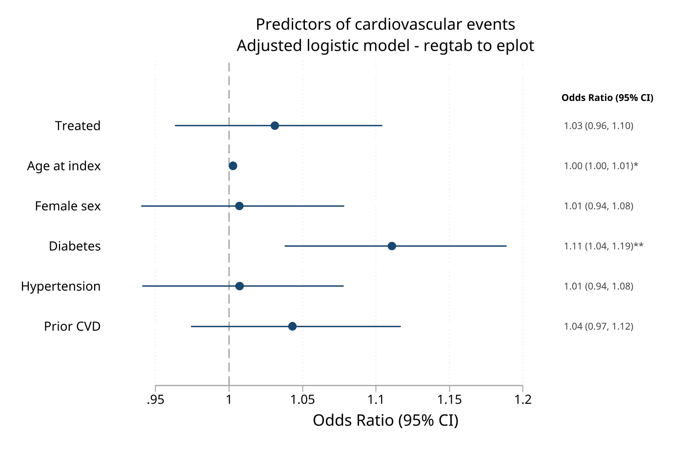
One model: regtab table, then eplot forest
regtab writes the table and the companion frame at once; eplot plots the frame.
collect clear
quietly collect: logistic cv_event treated index_age female diabetes hypertension prior_cvd
regtab, coef("OR") noint eplotframe(or_effects, replace) display

eplot, frame(or_effects) labels(label) rowtype(rowtype) ///
    null(1) values stars vformat(%4.2f) ///
    effect("Odds Ratio (95% CI)") ///
    title("Predictors of cardiovascular events")
The table:
  +-----------------------------------------------+
  |                Model                          |
  |                   OR         95% CI   p-value |
  |      Treated    1.03   (0.96, 1.10)      0.38 |
  | Age at index    1.00   (1.00, 1.01)     0.035 |
  |   Female sex    1.01   (0.94, 1.08)      0.84 |
  |-----------------------------------------------|
  |     Diabetes    1.11   (1.04, 1.19)     0.002 |
  | Hypertension    1.01   (0.94, 1.08)      0.84 |
  |    Prior CVD    1.04   (0.97, 1.12)      0.23 |
  +-----------------------------------------------+
The matching forest plot:
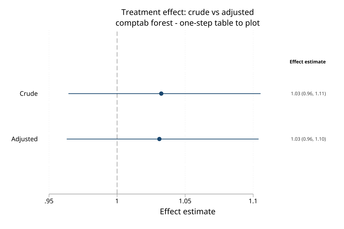
Several models: comptab forest in one step
comptab composes companion frames from multiple regtab runs; forest calls eplot for you, and eplotoptions() passes graph options through.
* Crude and adjusted treatment effects, each captured as a regtab frame
collect clear
quietly collect: logistic cv_event treated
regtab, coef("OR") noint frame(g_crude, replace) eplotframe(ge_crude, replace)

collect clear
quietly collect: logistic cv_event treated index_age female diabetes hypertension prior_cvd
regtab, coef("OR") noint frame(g_adj, replace) eplotframe(ge_adj, replace)

comptab g_crude g_adj, rows(1 \ 1) section("Crude" \ "Adjusted") ///
    forest eplotoptions(null(1) title("Treatment effect: crude vs adjusted"))
Resources
help tabtoolsfor the suite overview and persistent defaultstabtools_tipsorhelp tabtools_tipsfor compact option patterns and longer end-to-end recipeshelp tabtools_cheatsheetandhelp tabtools_cookbookas legacy aliases totabtools_tipshelp table1_tc,help desctab,help regtab,help effecttab,help comptab,help hrcomptab,help survtab,help stratetab,help crosstab,help corrtab,help diagtab,help puttab, andhelp stacktabfor command-specific syntax
Version History
- 1.6.4 (2026-06-10): Remove the retired workbook-composition alias from the shipped package.
stacktabis now the only public command for assembling exported workbook blocks, and QA no longer installs or calls the old alias path. - 1.6.3 (2026-06-10): Add
tabtools_tips, a merged quick-reference and cookbook command/help topic. The formertabtools_cheatsheetandtabtools_cookbookhelp files are retained as compatibility aliases. Update the visible help and README command inventory for recently added commands includingputtab,stacktab, andsimtab. - 1.6.2 (2026-06-08): Fix
regtabAIC/BIC for GEE models.regtabreads model fit statistics from the activee(), but Stata'sglm(the backend used byiivw_fitandxtgee-style GEE workflows) storese(aic)as AIC per observation (AIC/N) ande(bic)under a deviance-based convention — neither comparable to the likelihood-scale valuesmixedand other ML estimators report. Astats(aic)table mixing GEE and mixed models therefore showed GEE AIC values roughly N times too small.regtabnow always recomputes AIC as-2*ll + 2*kand BIC as-2*ll + k*ln(N)frome(ll),e(rank), ande(N)whenever those are available, overriding the per-observation/deviance-based stored values. Results now matchestat icfor every model family and stay on one scale across rows.mixedoutput is unchanged (it already used this path). Added regression testqa/regtab/test_regtab_aic_gee.do. - 1.6.1 (2026-06-08): Adds disk-backed tabtools defaults profiles.
tabtools set ... , permanentwrites the current house style to a runnable Stata do-file, usingtabtools_profile.doin the PERSONAL ado directory by default orprofile(filename)for project-specific profiles.tabtools use [using filename]reloads a saved profile into the current session, making fonts, themes, borders, digits, bold-p thresholds, and custom colors reproducible across sessions and projects. Refreshestable1_tcdisplay defaults toward a compact house style: continuous variables now useformat(%2.0f), percentagespercformat(%5.0f)with no percent sign (percsign("")), SDs render asmean±SD(sdleft("±") sdright("")), IQRs as(Q1, Q3)(iqrmiddle(", ")), and low percentages are reported without a leading alignment space (no-space is now the default — the old behavior is available via the newspacelowpercentoption, replacingnospacelowpercent).borderstyle(thin)is the default Excel border for bothtable1_tcandregtab, andregtabdefaults todigits(2). - 1.6.0 (2026-06-07): New command
simtab— a Monte Carlo simulation performance table and export layer. Compute mode summarizes long replication-level results into table-grade measures (mean,bias,pctbias,empse,meanse,relerr,mse,rmse,coverage,power,n,nonconv) with closed-form Monte Carlo SEs used to flag off-nominal coverage; ingest mode (from(simsum)/from(siman)/from(summary)) renders an already-computed summary without recomputation, following the optional-dependency pattern used bycomptab/hrcomptabwitheplot. Multi-estimand tables get merged Excel group headers and flattened Markdown/CSV headers;nsim()adds non-convergence reporting;plotframe()provides a numeric figure companion. Cross-validated to exact agreement withsimsumon bias/empirical SE/coverage and their Monte Carlo SEs. Pairs withsimsum(White, Stata Journal 2010) andsiman(UCL); cites Morris, White & Crowther (Stat Med 2019). Adds_simtab_ingest.ado,simtab.sthlp, andqa/simtab/. - 1.5.2 (2026-06-06): Cleaner forest plots from
comptabandhrcomptab. When asection()(or stratetab scaffold section) contributes exactly one plotted row, the eplot companion frame now folds the section label into that single row instead of emitting a standalone header row followed by one indented effect — the redundant header/child pair that made one-coefficient-per-model forests look cluttered. The rendered Excel and console tables are unchanged; only theeplotframe()/forestoutput differs. Addedqa/_package/test_eplot_section_fold.do. - 1.5.1 (2026-06-06): Fix two correctness bugs found while auditing the v1.5.0 eplot bridge.
comptabandhrcomptabcould not export Markdown (markdown()failed withrc=198because of a malformed compound quote in the post-forestreturn block).regtabdouble-exponentiatedlogit, orandologit, ormodels (thelogit/ologitbranch hardcodedeform=1instead of respecting a user-suppliedoroption, unlikemelogit/poisson/mlogit), silently reportingexp(OR); this also propagated into the eplot companion frame. Added regression tests for both inqa/_package/test_markdown_exports.doandqa/regtab/test_regtab_model_families.do. - 1.5.0 (2026-06-06): Add an
eplotbridge for graph-ready estimate/CI companion frames.regtabandeffecttabnow supporteplotframe();comptabandhrcomptabcan compose those companions and draw forest plots withforest, passing graph options througheplotoptions()while honoring the active graph scheme by default.regtabandeffecttabnow supporteplotframe();comptabandhrcomptabcan compose those companions and draw forest plots withforest, passing graph options througheplotoptions()while honoring the active graph scheme by default. - 1.4.0 (2026-06-05): Add
markdown()andmdappendexports across tabtools table commands, including same-call Excel plus Markdown export and sequential Markdown report building. Add_tabtools_markdown_write_current.adoas the shared Markdown writer and allowputtabto run Markdown-only withoutusing. - 1.3.7 (2026-06-03): Cap the label (first) column width in
regtab,effecttab, andcomptabso a single verbose row label — most commonly an unstructured random-effectsCovariance: ... (slope, Intercept)row from a mixed model — can no longer stretch the whole column to 60-76 characters and balloon the table. The label column now caps at 45 characters by default; labels longer than the cap wrap onto extra lines (top-aligned) instead of being clipped by the adjacent estimate cell. The cap is tunable via the newlabelwidth()option on all three commands. - 1.3.6 (2026-06-01): Add
puttab, a first-mile styled-block producer that writes a table already in memory — the current dataset, a namedframe(), or a Statamatrix()such ase(b),r(table), orcollapse/tabulateoutput — as one house-styled Excel sheet with the shared title/header/zebra/border geometry. For a matrix source the row and column names become the label column and header row; for a dataset or frame source numeric columns honordigits(), integers stay integer, and value labels are resolved. Repeated calls build a multi-sheet workbook thatstacktabcan assemble, closing the raw-input gap betweendesctab(needs acollect) andstacktab(needs pre-exported sheets). Addstacktabfor block assembly of composite sheets. Togetherputtabandstacktabform the emit-then-assemble export pipeline. - 1.3.5 (2026-06-01): Fix
effecttab, digits()so collect-rendered 95% CI bounds use the requested decimal precision. Addregtab, cutlabels()for ordered-model cutpoints, makenointhide cutpoint and ancillary-only rows such aslnalpha,alpha, and/sigma, and split model-family demos intodemo_regtab_models.xlsxwith richer zero-inflated examples. - 1.3.4 (2026-06-01): Extend
regtabmulti-equation row handling to zero-inflated Poisson, zero-inflated negative binomial, and Cragg hurdle models, with equation labels for outcome, inflation, selection, scale, and ancillary rows. Expand QA and demos for the model families covered by the regression-family matrix. - 1.3.3 (2026-05-31): Make
regtabpreserve multi-equation row identity for estimators such asmlogit, auto-display multinomial logit output as relative risk ratios (RRR), and add a regression-family QA matrix coveringmlogit, OLS, logit, probit, ologit, count, GLM, panel, survival, and quantile models. - 1.3.2 (2026-05-29): Make
regtab, stats()acceptn_subandsubjectsas synonyms forn(the N row, which already reports subjects for survival models), and warn instead of silently ignoring unrecognizedstats()tokens. - 1.3.1 (2026-05-27): Make
regtab, relabelrandom-effect rows identify variance and covariance parameters explicitly, including linear mixed-model random-slope covariance rows such ascov(months_since_tx,_cons). - 1.3.0 (2026-05-23): Replace final Excel writers with a shared Mata
xl()backend, add Mata workbook read/write helpers for collect parsing and backend contracts, and removeexport excel/import excelfrom command implementations. - 1.2.0 (2026-05-20): Add
regtab, nopvalueto suppress p-value columns from console, frame, CSV, and Excel and Markdown outputs while preserving internal p-values for significance stars and row highlighting. - 1.1.0 (2026-05-13): Add
desctab, a formatter for activetablecollections with per-statistic number formats,events / N (%)and other composite cells, Excel/CSV/frame/display outputs, and shared tabtools styling defaults. - 1.0.15 (2026-05-07): Fix
regtabICC cross-pollution where a multi-model collection ending inmepoisson/menbregsilently suppressed ICC for all earlier mixed-effects models (now skipped per-model). Strip thousands separators from coefficient and CI cells sodigits(),stars,boldp,dimnonsig, andr(table)work for coefficients ≥ 1000. Make reference-category detection match the underlying numeric value (0 or 1 with empty CI) instead of the rendered string, so non-default precision still labels rows "Reference". Emit a noisily warning when the per-model stats fallback fires for a multi-model collection. Documenttable1_tcreservedby()variable name prefixes (N_,m_,_c…). Plug a Mata workspace leak intable1_tcExcel error path. Use a tempname instead of the literalbeatlesvalue-label fallback. Replace ad-hoc…2suffix scratch columns inheaderpercwith tempvars to avoid name collisions. Move integer check beforerecast long, forceto prevent silent truncation. Sthlpboldpcolon-position fix. - 1.0.14 (2026-05-05): Add QIC (Quasi-likelihood Information Criterion) support to
regtabfor GEE models. Whenstats(aic)is requested afterxtgee, QIC is automatically computed and displayed since AIC is undefined for quasi-likelihood estimators. QIC can also be requested explicitly viastats(qic). - 1.0.13 (2026-04-27): Documentation improvements across all .sthlp files and README. Enhanced corrtab, survtab, and diagtab help files with richer descriptions, additional examples, and "Also see" sections. Standardized author blocks with mailto links. Added
{vieweralsosee}links to the cheatsheet. - 1.0.12 (2026-04-27): Fix
crosstab, or rr rdfor 2x2 variables coded with nonzero category values by internally recoding observed levels to 0/1 before calling Stata'scc/cs; reject undefined requested association measures instead of silently omitting them; and validatetable1_tcwt()and numericby()values within the analysis sample so excluded rows do not trigger false hard failures. - 1.0.11 (2026-04-26): Fix
table1_tc, wt() smdweighted SMD calculations for continuous, categorical, and binary variables; fixheaderpercwithtotal(before|after); and document activecollectside effects forregtabandeffecttab. - 1.0.10 (2026-04-26): Fix weighted
crosstab, trend, enforce unique truncatedstratetabmatrix row names, hard-fail missing finaleffecttabworkbooks, reject binarydiagtab, optimal, addcorrtabshape conflict checks, clarify cookbook runnable versus illustrative recipes, and strengthen QA/install isolation. - 1.0.9 (2026-04-23): Fix
regtabexporting a spurious blank trailing column. The_re_group_labelinternal variable was not being dropped before export because it was bundled in acapture dropwith_ci_seen, which only exists underdimnonsig. - 1.0.8 (2026-04-22): Clarity audit release with hardened export-return behavior, synchronized package metadata, and expanded QA around release gates and export failures.
- 1.0.7 (2026-04-18): Stata-Tools suite release covering direct descriptive tables,
collect-based model formatters, file-based rate workflows, and frame-based composite builders. - 1.0.6 (2026-04-17): Incremental refinement release during the Stata-Tools packaging cycle.
- 1.0.5 (2026-04-17): Incremental refinement release during the Stata-Tools packaging cycle.
- 1.0.4 (2026-04-16): Early public packaging milestone for the tabtools suite.
Author
Timothy P Copeland, Karolinska Institutet